Lucy's Algorithm + Fenwick Trees
Abstract. I describe how Lucy_Hedgehog’s algorithm works, and how it can be implemented. Then I show how Fenwick trees can be used to boost its runtime without much effort. The final runtime is at most $O(x^{2/3} (\log x)^{1/3})$ to compute $\pi(x)$.
I also give an extension to sums of primes and to primes in arithmetic progressions.
The implementation gives $\pi(10^{13})$ in less than 3s.
There are a lot of nice combinatorial algorithms for computing $\pi(x)$, the number of primes $p \leq x$. One very commonly implemented algorithm is the Meissel-Lehmer algorithm, which runs in roughly $O(x^{2/3})$ time and either $O(x^{2/3})$ or $O(x^{1/3})$ space depending on if you go through the trouble to do segmented sieving, which can be complicated.
In fact many expositions of the ML algorithm that I’ve seen look awfully complicated. This exposition by Lagarias, Miller, and Odlyzko gives a lot of detail for those who wish to try implementing it. I haven’t tried myself yet. Mostly because the method I’m going to detail in this post has proven completely sufficient for me and simpler to write.
The purpose of this post is to talk about arguably the simplest efficient prime counting algorithm out there - it is nowhere near the fastest (and there are lots of cool ways to do this), but it is very fast. In the end we’ll be able to compute $\pi(10^{13})$ in less than 3s. If you want the absolute fastest prime counting algorithm, you’ll have to look at some more complicated math than this - I think it’s generally accepted that Kim Walisch’s primecount contains some of the fastest implementations of some very technically complex algorithms for this purpose. Check it out even if you aren’t implementing those algorithms yourself.
I’ll be describing how the basic algorithm works first, and then showing how you can use a Fenwick tree to asymptotically improve the runtime by using some more memory. This is a long and involved read with a lot of references, but I’ve tried my best to be accurate and descriptive here. I’m going to write this assuming that the reader hasn’t seen either Lucy’s algorithm nor Fenwick trees before.
I added an addendum today, Feb 10 2025, mentioning some implementation improvements that were preventing my basic Lucy’s algorithm from being fast. Please read it at some point along the way.
Throughout, $x$ will be the large integer (like $10^8 \ll x \ll 10^{15}$) for which we want to calculate $\pi(x)$.
The Lucy_Hedgehog Algorithm
Named for Project Euler user Lucy_Hedgehog, this was actually originally an algorithm to compute the sum $\sum_{p \leq x} p$. You can find their original post about this in the forum threads for problem 10. The idea is to describe what happens in a sieve of Eratosthenes and use what some more people call the “square root trick”.
In the sieve of Eratosthenes, one starts by initializing every integer from $2$ to $x$ as “maybe prime”.
The smallest element in the sieve is now marked as definitely prime, and all of its multiples are eliminated from the sieve. This is repeated until all primes have been yanked out. If you couldn’t write one of these sieves from memory, it would probably be helpful to your understanding to do some research into it, as Lucy’s algorithm and the Eratosthenes sieve are conceptually very similar.
So, for each prime $p \leq x$, we would be iterating over all of its multiples, which gives us basically a runtime of $\sum_{p \leq x} \frac{x}{p} \sim x \log \log x$ (check out Mertens’ second theorem if this is unfamiliar).
To turn this into a nice prime counting algorithm we define a function $S(v, p)$ which will be the number of integers $n$ in the range $2 \leq n \leq v$ remaining after sieving with all of the primes up to $p$. We start with $S(v, 1) = v-1$ since $1$ is never in the sieve.
Considering $S(v, p)$, we see that every integer we eliminate from the sieve is a multiple of $p$. Specifically (and you should check this by doing the sieve by hand!) the integers we eliminate are $p*n$ where $n$ are the integers remaining in the sieve that are between $p$ and $v/p$.
This leads us to the crucial formula
\[S(v, p) = S(v, p-1) - \left[S(v/p, p-1) - S(p-1, p-1)\right]\]One more very important observation is that if $p^2 > v$, then $S(v, p) = S(v, p-1)$ - that is, we only actually need to sieve out the primes up to $\sqrt{v}$, after which we will have $S(x, \sqrt{x}) = \pi(x)$.
Square Root Trick
The next important theoretical detail on the list relates to the “key values” $v$ which show up as arguments in a recursive implementation of $S(v, p)$. Since $S(v, p) = S(\lfloor v \rfloor, p)$, we should only consider integer arguments.
Part of the story here is the equality
\[\left \lfloor \frac{\lfloor x/m \rfloor}{n} \right \rfloor = \left \lfloor \frac{x}{mn} \right \rfloor\]You should convince yourself of this - the left hand side is the largest integer $k$ such that $kn \leq \lfloor x/m \rfloor$. This is true if and only if $kn \leq x/m$, for which $k$ is maximized at $\left \lfloor \frac{x}{mn} \right \rfloor$.
So, with this knowledge in mind, each key value $v$ is just the floor of a bigger key value divided by an integer - hence the set of key values is the set of distinct values taken by $\left \lfloor \frac{x}{n} \right \rfloor$.
The “square root trick” describes exactly how many and which values that expression can take. It’s closely related to Dirichlet’s hyperbola method (described in this blog post and in section 3.5 of Apostol’s Introduction to Analytic Number Theory). The idea is that if $n \leq \sqrt{x}$, all of the values $\lfloor x/n \rfloor$ will be distinct, and if $n > \sqrt{x}$ we will have $\lfloor x/n \rfloor < \sqrt{x}$. Therefore there are at most $2\sqrt{x}$ distinct key values to deal with, which is not so bad.
The following image shows a plot of $10/n$ (the blue line) and the values $\lfloor 10/n \rfloor$ as black points. The blue shaded section is for $n \leq \sqrt{10}$, and you can see that for $n > \sqrt{10}$ we have lots of repeated values due to the restriction $10/n \leq \sqrt{10}$.
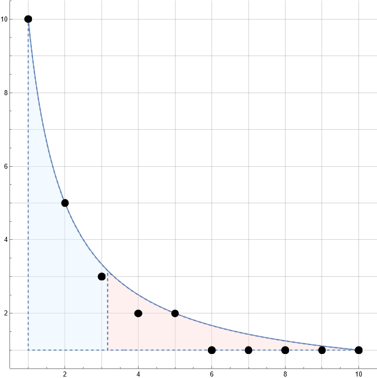
This trick is ubiquitous and used in a large variety of number theoretic summation techniques, for example in this algorithm to compute the partial sums of the totient function $\varphi(n)$ in $O(x^{3/4})$ time1.
Data Structure Details
To implement Lucy’s algorithm, then, it helps to have a nice container to store an int64 at each key value v (where x is fixed and known). In my personal library I use a lightweight wrapper object which stores the following data:
- The value
x - The value
isqrtdefined as $\lfloor \sqrt{x} \rfloor$ - An array
arrof lengthL, where $L = 2\lfloor \sqrt{x} \rfloor$, or if $\left\lfloor \frac{x}{\lfloor \sqrt{x} \rfloor}\right\rfloor = \lfloor \sqrt{x}\rfloor$ use $L = 2\lfloor \sqrt{x} \rfloor-1$ - An array
keysof lengthL, which contains in increasing order the different values of $\lfloor x/n \rfloor$.
The array of keys was added in February 2025. Please see the addendum.
We will see why we sometimes need this lower value of L presently.
The strategy is to use keys = 1, 2, ..., isqrt, x div isqrt, x div (isqrt-1), ..., x as indices.
This has a total length of 2*isqrt. If we query the input v, we check if v <= isqrt. If it is, we return arr[v-1], and otherwise return arr[L-(x div v)].
For example, with $x = 12$ we have isqrt == 3 and our array elements correspond to
No issues here. Let’s try with $x = 10$, where isqrt == 3 again, but
This duplicate index would cause us a headache. Hence if at the boundary we have isqrt == x div isqrt we will omit that second value, giving us L == 2*isqrt - 1 in that case. It’s important to be careful about this both here and in other applications of the square root trick.
In the code, I’ll be calling this container FIArray - standing for floor indexed array. There’s no actual name for this but this one seems as good as any. Here’s a simple implementation2 in Nim (note that div is floor division):
import iops, tables

##Given x, store the different values floor(x/n) in increasing order
var keysTableFI = initTable[int64, seq[int64]]()

proc keysFI*(x: int64): seq[int64] =
  if keysTableFI.hasKey(x): return keysTableFI[x]
  #generate key table for the first time
  let rt = isqrt(x)
  result = @[]
  for v in 1..rt: result.add v
  if rt != x div rt:
    result.add x div rt
  for n in countdown(rt - 1, 1):
    result.add x div n
  #save it in case we want to use these keys again later
  keysTableFI[x] = result

type FIArray* = object
  ##Given x, stores a value at each distinct (x div n).
  x*: int64
  isqrt*: int64
  arr*: seq[int64]
  #keys is accessed by keysTable[x]

proc newFIArray*(x: int64): FIArray =
  ##Initializes a new FIArray with result[v] = 0 for all v.
  result.x = x
  var isqrt = isqrt(x)
  result.isqrt = isqrt
  var L = 2*isqrt
  if isqrt == (x div isqrt): dec L
  result.arr = newSeq[int64](L)

proc indexOf*(S: FIArray, v: int64): int =
  ##Computes the index of key value v in S.arr, using a division.
  ##Try NOT to need to use this, as divisions are very slow.
  if v <= S.isqrt: return v-1
  return S.arr.len - (S.x div v)

proc `[]`*(S: FIArray, v: int64): int64 =
  ##Accesses S[v], using a division.
  if v <= 0: return 0
  if v <= S.isqrt: return S.arr[v-1]
  return S.arr[^(S.x div v).int] #equiv S.arr[L - (S.x div v)]

proc `[]=`*(S: var FIArray, v: int64, z: int64) =
  ##Sets S[v] = z, using a division.
  if v <= S.isqrt: S.arr[v-1] = z
  else: S.arr[^(S.x div v).int] = z
Nothing magical is happening here quite yet, it’s just incredibly helpful to have these functions set up when we actually implement Lucy’s algorithm. Speaking of, we can describe and implement it now -
Algorithm (Lucy)
- Initialize
S[v] = v-1for each key valuev.- For
pin2..sqrt(x),
2a. IfS[p] == S[p-1], thenpis not a prime (why?) so incrementpand try again.
2b. Otherwise,pis a prime - for each key valuevsatisfyingv >= p*p, in decreasing order, update the value atvbyS[v] -= S[v div p] - S[p-1].- Return
S. Here,S[v]is the number of primes up tovfor each key valuev.
Why, in step 2b, do we have to update the array elements in decreasing order?
This is a side effect of us using a single array S to store S[v, p] for all keys v and p <= isqrt. There is a loop invariant here: after step 2b, S[v] = S[v, p]. During step 2b, part of the array should be S[v, p] and part of it should be S[v, p-1]. We have to be careful that when we update S[v] to equal S[v, p] that we will not need the value S[v, p-1] in the future, since it will be overwritten. The natural way to make sure of this is to simply update the highest v first, since any S[v, p] will only need to access S[w, p-1] for w < p.
I’m not sure if my explanation of this part in words is completely satisfactory, so here I’ve3 drawn a small dependency graph of S[v, p] for x = 10.

We see that each S[v, p] depends only on S[w, p-1] for w <= v.
Also notice the curious S[5, 2] node which is not actually used to compute S[10, 3] - we can skip some work by not updating S[5, 2] at all! That’s not immediately relevant but it is a key part of some algorithms which do not produce every value $\pi(v)$ and only produce a provably correct value of $\pi(x)$.
For now, though, here’s the incredibly simple Nim implementation of Lucy’s algorithm:
proc lucy(x: int64): FIArray =
  var S = newFIArray(x)
  var V = keysFI(x)
  for i, v in V.pairs:
    S.arr[i] = v-1 #set S[v] = v-1
  for p in 2..S.isqrt:
    #since p is small we have
    #S[p] = S.arr[p-1], S[p-1] = S.arr[p-2]
    if S.arr[p-1] == S.arr[p-2]: continue
    #p is prime
    let sp = S.arr[p-2] #= S[p-1]
    for i in countdown(V.len - 1, 0):
      let v = V[i]
      if v < p*p: break
      #S[v] = S[v] - (S[v div p] - S[p-1])
      S.arr[i] = S.arr[i] - (S[v div p] - sp)
  return S
Again see the addendum for mention of a small change that’s been made here.
Hopefully you can understand the allure of this prime counting method.
A quick benchmark tells us that we can compute $\pi(10^{12}) = 37607912018$ in only 2.2s (on my machine). Since we only store about $2\sqrt{x} = 2*10^6$ values in our container, this also has fantastic memory usage. If we try running it at a few more powers of ten we get the following runtime data:
| x | pi(x) | Time (s) |
|---|---|---|
| 109 | 50847534 | 0.016 |
| 1010 | 455052511 | 0.08 |
| 1011 | 4118054813 | 0.41 |
| 1012 | 37607912018 | 2.2 |
| 1013 | 346065536839 | 11.4 |
| 1014 | 3204941750802 | 60.1 |
Beyond $10^{14}$ we’re a little too lazy to wait so long. Honestly, the algorithm described so far probably suffices for most uses in Project Euler, and even for $10^{14}$ you only need an array of length $2*10^7$ which is very reasonable. In Lucy’s original post, they add that it “is also possible to improve the complexity of the algorithm… but the code would be more complex”. In the paper of Lagarias, Miller and Odlyzko, mention is made to a “special data structure” which is key to achieving a faster runtime. Both of these are referring to a Fenwick tree, a structure which allows efficient prefix sums and array updates. The inclusion of a Fenwick tree will significantly increase memory requirements, from $O(\sqrt{x})$ to $O(x^{2/3})$ or so, but it will also give us a nice performance boost.
Runtime Analysis
This section is really short because this is actually pretty easy.
For each prime $p \leq \sqrt{x}$ we need to do an array operation for each key value $v \geq p^2$. We’ll count the contribution of primes with $p^2 \geq \sqrt{x}$ and those with $p^2 < \sqrt{x}$ separately.
There are at most $x^{1/4}$ small primes, and for each of them we need to do $O(\sqrt x)$ array updates, for a total runtime contribution of $O(x^{3/4})$.
For the large primes $p$, there are at most about $\frac{x}{p^2}$ key values to look at (check this!4), for a total runtime contribution of
\[\begin{align*} \sum_{x^{1/4} \leq p \leq \sqrt{x}} \frac{x}{p^2} &\leq \sum_{x^{1/4} \leq k} \frac{x}{k^2}\\ &\leq \frac{x}{(x^{1/4})^2}+ x \int_{x^{1/4}}^\infty \frac{dt}{t^2}\\ &\leq \sqrt{x} + x^{3/4} \end{align*}\]And so the runtime of Lucy’s algorithm is $O(x^{3/4})$!5
Fenwick / Binary Indexed Trees
If you haven’t scrolled down and read the addendum please do so now.
A Fenwick Tree (also known as a Binary Indexed Tree or BIT) is a data structure which has been described in a billion different places in a lot of detail by very smart computer scientists who know a lot more than I do. Really - this thing has a plethora of uses, for example counting inversions in an array, quickly calculating the index of a permutation among all permutations listed lexicographically6, and as you’ll see soon, prime counting! Seriously, you should go read all the articles I just linked.
I’m only going to be lightly touching on how a Fenwick tree works, because I’d rather just use it as a black box here.
Suppose we have an array a[1..n] indexed from 1 to n.
A standard Fenwick tree supports two operations:
- Prefix sums, which query
a[1] + a[2] + ... + a[i]for somei <= n. - Updates, which modify the array by
a[i] += cfor somei <= nand integerc.
On an ideal array, the first operation would take $O(i)$ time, and the second would take constant time.
In our applications we would like to perform the prefix sums quickly. One idea is to store the prefix sums instead of the base array - that way we can get the prefix sums in constant time. But then to update an element of the array we would have to modify $O(n-i+1)$ partial sums, and so the update operation gets as slow as the prefix operation once was.
A Fenwick tree balances the prefix and update operations - both will take $O(\log n)$ time, which is excellent.
The way this is done is by computing a bunch of range sums over many different overlapping intervals of the base array. It’s done in such a way that
- every prefix sum is composed of $O(\log n)$ of the intervals we have pre-computed, and
- every element of the base array belongs to $O(\log n)$ of the intervals we care about!
Thus, if we want to compute a prefix sum we just add up $O(\log n)$ values, and to update an element of the base array we update $O(\log n)$ range sums.
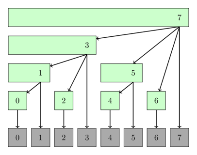
Image source is cp-algorithms.com.
It’s all very nice in theory but sounds like it would be a bit annoying to implement. Fortunately you can essentially use the binary structure of computer memory to your benefit, which makes it exceptionally simple to code:
type Fenwick[T] = object
  arr: seq[T]

proc newFenwick[T](len: int): Fenwick =
  result.arr.newSeq(len)

proc len[T](f: Fenwick[T]): int = f.arr.len

proc sum[T](f: Fenwick[T], i: SomeInteger): T =
  ##Returns f[0] + f[1] + ... + f[i]. Time O(log i).
  var ii = i+1 #uses 1-indexing for bit tricks
  while ii>0:
    result += f.arr[ii-1]
    ii -= (ii and (-ii))

proc addTo[T](f: var Fenwick[T], i: SomeInteger, c: T) =
  ##Adds c to a single element of the base array. O(log i)
  var ii = i+1 #uses 1-indexing for bit tricks
  while ii<=f.arr.len:
    f.arr[ii-1] += c
    ii += (ii and (-ii))

proc `[]`[T](f: Fenwick[T], i: SomeInteger): T =
  ##Accesses a single element of the base array. O(log i)
  if i==0: return f.sum(0)
  return f.sum(i) - f.sum(i-1)

proc `[]=`[T](f: var Fenwick[T], i: SomeInteger, x: T) =
  ##Sets a single element of the base array. O(log i)
  f.addTo(i, x-f[i])
This is a basic, barebones implementation of the structure, but it’ll work great.
I’ve also given it a generic type T, which will be int in our case. It’s helpful to be able to use int64 in case you want to do sums of primes later (you do).
It’s possible to do a lot more than this with a Fenwick tree. For example, if you have a nontrivial initial state you’d like the base array to have, you can initialize the tree in linear time instead of updating each of the elements individually. It’s explained in this Codeforces blog by sdnr1.
For ease of use I’m going to use a slightly less general version of that method in which we create the Fenwick tree with a default value - every element of the base array equal to some constant default.
It looks like this:
proc newFenwick[T](len: int, default: T): Fenwick[T] =
  ##Initializes a fenwick tree with a constant array, f[i] = default for all i.
  result.arr.newSeq(len)
  for i in 0..<len:
    result.arr[i] = default
  for i in 1..len:
    var j = i + (i and (-i))
    if j<=len:
      result.arr[j-1] += result.arr[i-1]
This is everything we need from the land of data structures to speed up Lucy’s algorithm.
Application of Fenwick Trees to Lucy’s Algorithm
The way we trade memory for speed here is common to algorithms of this type.
Select some constant $\sqrt{x} < y \leq x$ as a parameter to be optimized later. We will be performing a standard Eratosthenes sieve up to $y$ while updating our FIArray using the recursion we derived earlier for the key values $v > y$. If you’ve seen some of the faster methods for computing the totient summatory function, this will seem familiar. I am going to describe the algorithm next, and we will discover why Fenwick trees are needed here.
Initialize the Eratosthenes sieve as usual with all of the numbers from 2 to y marked as “maybe prime”. At the same time initialize the FIArray for Lucy’s algorithm as usual. Now for each of the $O(x/y)$ key values satisfying $v \geq y$ update the FIArray in the same way as in Lucy’s algorithm. We will then proceed with a step of the sieve - identifying a prime p and eliminating all of its multiples from the sieve in $O(y/p)$ time.
The important bit to note here is that if the Lucy step sets S[v, p] -= S[v div p, p-1] - S[p-1, p-1] and either of v div p or p-1 is at most y, then instead of using the value stored in the FIArray we need to compute the number of remaining integers in the Eratosthenes sieve. This is the application of the Fenwick tree - we can store a 1 if the integer is maybe prime and a 0 if it is definitely not prime, and then prefix sums compute the number of remaining integers up to some value.
Now that we know what’s going to happen, here’s the algorithm:
Algorithm (Lucy + Fenwick)
- Compute the sieving limit $y$.
- Initialize a Fenwick tree called
sieveindexed on0..y, with default value1.
Setsieve[0]andsieve[1]to0, since these are not a part of the initial Eratosthenes setup.- Initialize a boolean array
sieveRawin a similar way assieve- initialized tofalse, and then setsieveRaw[0]andsieveRaw[1]totrue. It’s a little easier to have it inverted in this way, wheresieveRaw[j]beingtruecorresponds tojbeing composite. This has very little impact on space requirements and will allow us to query a single element of the base sieve array in constant time which will be helpful.- For
pin2..sqrt(x),
4a. IfsieveRaw[p]istrue, thenpis not a prime so incrementpand try again.
4b. Otherwise,pis a prime - for each key valuevsatisfyingv >= p*pandv > y, in decreasing order, update the value atvbyS[v] -= S_0[v div p] - S_0[p-1], whereS_0[u]is equal toS[u]ifu > yand equal tosieve.sum(u)otherwise.
4c. Do a step of the Eratosthenes sieve - for each multiple ofpup toy, sayj = p*k, checksieveRaw[j]. If it isfalse, we need to eliminatejfrom the sieve by settingsieveRaw[j]totrueand adding-1tosieve[j].- For each key value $v \leq y$, set
S[v] = sieve.sum(v).- Return
S. Here,S[v]is the number of primes up tovfor each key valuev.
Analysis + Optimization
Updated 5/2/2023.
Clearly we are using $O(y)$ space. So how about our runtime?
This part will involve a lot of tedious casework so feel free to skip it and trust me instead.
For each prime $p \leq \sqrt{x}$, the Eratosthenes step has to modify sieve[p*k] whenever p*k needs to be marked as composite. Thus we need to update the Fenwick tree at n once for each composite $n \leq y$.
Each update using the Fenwick tree takes $O(\log(y))$ time.
Then the Eratosthenes step takes us a total runtime of
\[O\left(\sum_{n \leq y} \log(y)\right) = O\left(y \log y\right)\]Okay, now for the Lucy step. Here I won’t aim for a perfect asymptotic but will be alright with an upper bound to avoid the most headache inducing analysis. Feel free to be more precise on your own.
The analysis will be slightly different depending on whether $p^2 \leq y$.
If it is one of these small primes, then for each key value $v > y$ we need to do at most $O(\log y)$ work to update the FIArray at v. Since there are about $x/y$ such key values, this is a total time of (at most)
Now if instead $p$ is a big prime with $p^2 > y$, we will have to update only the key values with $v \geq p^2$, with a total time of (at most)
\[\sum_{\sqrt{y} < p \leq \sqrt{x}} \frac{x}{p^2} \log(y) \sim x \log(y) \sum_{\sqrt{y} < p \leq \sqrt{x}} \frac{1}{p^2}\]Now we want to get a decent estimate on that inverse prime sum. It’s actually a lot simpler than it seems, since we can upper bound it very lazily by
\[\begin{align*} \sum_{\sqrt{y} < p \leq \sqrt{x}} \frac{1}{p^2} & \leq \sum_{\sqrt{y} < p} \frac{1}{p^2}\\ & \leq \sum_{\sqrt{y} < n} \frac{1}{n^2}\\ &= O\left( \int_{\sqrt{y}}^\infty \frac{1}{t^2}dt \right) = O\left(\frac{1}{\sqrt{y}}\right) \end{align*}\]So in total the Lucy part of the algorithm takes a runtime of at most
\[O\left(\frac{x}{\sqrt{y}}\right) + O\left(\frac{x \log y}{\sqrt{y}}\right) = O\left(\frac{x \log y}{\sqrt{y}}\right)\]Our laziness in that last estimate is clear here. If we’re more careful and use (for example) Abel’s summation theorem along with estimates on $\pi(t)$ for $t \leq x$ we can get a clearer idea of how that second sum behaves. If we apply it to the sum $\sum_{p > \sqrt{y}} \frac{1}{p^2}$ we obtain
\[\sum_{p > \sqrt{y}} \frac{1}{p^2} = -\frac{\pi(\sqrt{y})}{y} + \int_{\sqrt{y}}^\infty \frac{\pi(t)}{t^3}dt\]Using the estimate $\pi(t) = O(t/\log(t))$ we’re going to prove that
\[\sum_{p > \sqrt{y}} \frac{1}{p^2} = O\left(\frac{1}{\sqrt{y} \log \sqrt{y}}\right)\]which will be an excellent estimate.
The first term is trivial, just plug in the estimate of $\pi(\sqrt{y})$ as follows:
\[-\frac{\pi(\sqrt{y})}{y} = O\left(\frac{\sqrt{y}}{y \log \sqrt{y}}\right) = O\left(\frac{1}{\sqrt{y} \log \sqrt{y}}\right)\]For the second one, plugging the estimate in yields
\[\begin{align*} \int_{\sqrt{y}}^\infty \frac{\pi(t)}{t^3}dt &= O\left(\int_{\sqrt{y}}^\infty \frac{1}{t^2 \log t}dt\right)\\ &= O\left(\frac{1}{\log \sqrt{y}}\int_{\sqrt{y}}^\infty \frac{1}{t^2}dt\right)\\ &= O\left(\frac{1}{\sqrt{y} \log \sqrt{y}}\right) \end{align*}\]So then finally we can plug this back into our estimate on the contribution of the big primes to show that they too only contribute $O\left(\frac{x}{\sqrt{y}}\right)$ to the final runtime in the Lucy section - nice!
Alright, so putting this all together now:
- The Eratosthenes section takes at most $O(y \log y)$ time
- The Lucy section takes at most $O\left(\frac{x}{\sqrt{y}}\right)$ time
We want to choose $y$ to balance these out. To do this we can pick $y$ proportional to
\[\frac{x^{2/3}}{(\log x)^{2/3}}\]I’m not guaranteeing this is optimal, especially since my analysis gave a lot of slack.
It should be fine though - the final runtime with this value of $y$ should be at least as good as
Not bad really! You’ll have to tune the value of $y$ in your own impementation, probably by multiplying by a constant or something. This is where you get to use some trial and error. I’ve found using about 0.35 times the value I stated works fine.
Finally we can implement this in Nim! Here’s how it looks.
proc lucyFenwick(x: int64): FIArray =
  var S = newFIArray(x)
  #compute y
  var xf = x.float64
  var y: int
  if x == 1: y = 1
  else:
    y = round(0.35*pow(xf, 2.0/3.0) / pow(ln(xf), 2.0/3.0)).int
    y = min(y, 4e9.int) #upper bound - set this depending on how much ram you have
    y = max(S.isqrt.int+1, y) #necessary lower bound
  var sieveRaw = newSeq[bool](y+1)
  var sieve = newFenwick[int](y+1, 1) #initialized to 1
  sieveRaw[1] = true
  sieveRaw[0] = true
  sieve[1] = 0
  sieve[0] = 0

  let V = keysFI(x)
  for i, v in V.pairs:
    S.arr[i] = v-1

  proc S0(v: int64): int64 =
    #returns sieve.sum(v) if v <= y, otherwise S[v].
    if v<=y: return sieve.sum(v.int)
    return S[v]
  for p in 2..S.isqrt:
    if not sieveRaw[p]:
      #right now: sieveRaw contains true if it has been removed before sieving out p
      var sp = sieve.sum(p-1) #compute it only once
      var lim = min(x div y, x div (p*p))
      for i in 1..lim:
        S.arr[^i.int] -= S0(x div (i*p)) - sp
        #here, S.arr[^i] = S[x div i] is guaranteed due to the size of i.
      var j = p*p
      while j <= y:
        if not sieveRaw[j]:
          sieveRaw[j] = true
          sieve.addTo(j, -1)
        j += p
  for i, v in V.pairs:
    if v>y: break
    S.arr[i] = sieve.sum(v)
  return S
Benchmarks
At last we’re through the derivation and implementation. Let’s see how it runs!
The following table includes the old runtimes for comparison.
| x | Lucy (s) | Lucy + Fenwick (s) |
|---|---|---|
| 109 | 0.016 | 0.014 |
| 1010 | 0.08 | 0.07 |
| 1011 | 0.41 | 0.30 |
| 1012 | 2.2 | 1.4 |
| 1013 | 11.4 | 6.9 |
| 1014 | 60.1 | 33.8 |
It’s of note that the new algorithm, although using more memory, only uses about 1GB for $10^{14}$.
If we’re willing to temporarily sacrifice 4GB of ram and permanently sacrifice three minutes of our lives we can push this new algorithm to calculate $\pi(10^{15}) = 29844570422669$. In the implementation I gave I include a cap on $y$ to restrict memory usage, so we could push this to ask for $\pi(10^{16})$ or $\pi(10^{17})$ and get an answer in a relatively reasonable amount of time.
Sums of Primes, Primes Squared, …
For these remaining few sections, rather than going in depth like the previous ones I’m just going to give a summary overview to wrap things up. What I want to talk about now is adapting this algorithm to sum functions of primes $f(p)$ where $f$ is nice. There are some nice ways to do this when $f$ has a particular form - for example if $f$ is a completely multiplicative function, ecnerwala describes a cool algorithm in the comments of this blog post. Here, we’ll show that if we can compute partial sums of $f(n)$ quickly, and $f(n)$ is completely multiplicative, then we can compute $\sum_{p \leq x} f(p)$ using Lucy’s algorithm. Moreover, as we would hope, we can also speed these up with Fenwick trees.
First let’s describe the difference in the plain Lucy algorithm.
Instead of a standard Sieve of Eratosthenes, we’ll be initializing the sieve array to $f(v)$ for $2 \leq v \leq x$. As we sweep $p$ from $2$ to $\sqrt{x}$, we will know $p$ is prime if the value at place $p$ is equal to $f(p)$. And if so, we’ll be eliminating the values $f(pk)$ for the multiples of $p$ that remain. Let’s copy and paste our explanation from the original Lucy algorithm and see what we have to change…
To turn this into a nice prime counting summing algorithm we define a function $S_f(v, p)$ which will be the number of integers sum of $f(n)$ over the remaining $n$ in the range $2 \leq n \leq v$ after sieving with all of the primes up to $p$. We start with $S_f(v, 1) = f(2) + f(3) + \ldots + f(v)$ since $1$ is never in the sieve.
Remembering from before that the integers we eliminate while sieving out $p$ for $S_f(v, p)$ are exactly $p*n$ where $n$ are the integers remaining in the sieve that are between $p$ and $v/p$, we have
\[S_f(v, p) = S_f(v, p-1) - f(p)\left[S_f(v/p, p-1) - S_f(p-1, p-1)\right]\]Lucy’s original post on this uses $f(n) = n$ for all $n$, since they were summing primes rather than counting them. Assuming we can quickly sum these $f$ in order to get our initial values, the plain algorithm works just fine and will give you whatever sum you want.
How about the Lucy + Fenwick algorithm? Well, there’s not any issue there either - we have to initialize the sieve so that sieve[i] = f[i], which is fine, and we have to use the slightly modified recursion for $S_f(v, p)$, but nothing else really changes. Trying to make this generic is a fun weekend project.
Primes in Arithmetic Progressions
Dirichlet considered the problem of computing the number of primes in a given arithmetic progression - that is, computing the number of primes in the sequence $a, a+d, a+2d, \ldots$ below $x$.
We’ll write $\pi_{d,a}(x)$ for this quantity.
In Dirichlet’s famous theorem on arithmetic progressions, he proved that each $\pi_{d,a}(x)$ tends to infinity as $x$ gets large, so long as $d$ and $a$ don’t share any factors (whence all large values of $a, a+d, a+2d, \ldots$ will be composite). To do this, he used what are called Dirichlet characters - complex valued, completely multiplicative, periodic functions $\chi(n)$.
Given that these characters $\chi$ are periodic and completely multiplicative, they fit our rule for when we can compute $\sum_{p \leq x} \chi(p)$ nicely - they pose no problem other than being complex floats instead of integers.. actually.. that’s very annoying. We’ll ignore that for a moment and see how we would continue.
Consider the set of all $\varphi(d)$ characters which have period $d$ (just trust me if you don’t know what I’m talking about).
We can compute the following sum in about $O(\varphi(d)x^{2/3}(\log x)^{1/3})$ time:
\[\begin{align*} \frac{1}{\varphi(d)} \sum_\chi \overline{\chi}(a) \sum_{p \leq x} \chi(p) \end{align*}\]Here, $\overline{\chi}$ is the complex conjugate of $\chi$. The reason this is nice is that we can actually switch the order of summation:
\[\begin{align*} \frac{1}{\varphi(d)} \sum_{p \leq x} \sum_\chi \overline{\chi}(a) \chi(p) \end{align*}\]The orthogonality relations for Dirichlet characters give us
\[\sum_\chi \overline{\chi}(a) \chi(p) = \begin{cases}\varphi(d) & \text{if } p \equiv a \bmod d\\ 0 &\text{otherwise}\end{cases}\]So our sum actually simplifies to $\pi_{d,a}(x)$.
It sucks to work with complex numbers though - and it’s possible to avoid the use of Dirichlet characters entirely by modifying the Lucy algorithm outright.
We will have one Eratosthenes sieve for each of the $\varphi(d)$ possible reduced residues mod $d$ - for example if $d = 6$ we will have one sieve containing all of the integers congruent to $1$ mod $6$, and another for all of the integers congruent to $5$ mod $6$.
In Lucy’s algorithm this would mean instead of having a single FIArray called S, we would have a set of $\varphi(d)$ of them. Let’s call them $S_{d,a}(v, p)$ for the $\varphi(d)$ relevant values of $a$. The tricky part here is figuring out how sieving works here.
Say we’re sieving out the prime $p$. Compute its inverse $p^{-1} \bmod d$. The integers we’re sieving out from $S_{d,a}$ will be multiples of $p$, say each one is written as $pk$. Then $k \equiv ap^{-1} \bmod d$ gives us the sieve that each $k$ will belong to! This way, the nice recursion from Lucy’s algorithm turns into…
\[S_{d,a}(v, p) = S_{d,a}(v, p) - \left[S_{d,ap^{-1}}(v/p, p-1) - S_{d,ap^{-1}}(p-1, p-1)\right]\]We have to initialize each $S_{d,a}(v,1)$ to be the number of integers in the progression $a, a+d, \ldots$ up to $v$, and be careful to subtract $1$ from $S_{d,1}(v,1)$ since we still don’t want $1$ to be included at the start. It’s a little bit more work but not too bad. It could look like this:
proc lucyAP(n: int64, k: int): seq[FIArray] =
  #find reduced residues
  var cop: seq[int] = @[]
  var ci = newSeq[int](k) #ci[v] = index of v in cop if gcd(v, k) = 1
  for i in 1..k-1:
    if gcd(i, k)==1:
      cop.add(i)
      ci[i] = cop.high
  #cop has size phi(k)

  var pis = newSeq[FIArray](cop.len)
  let V = keysFI(n)
  for i in 0..cop.high:
    pis[i] = newFIArray(n)
    for j, v in V.pairs:
      pis[i].arr[j] = (v - cop[i] + k) div k
      if i == 0: pis[i].arr[j] = pis[i].arr[j] - 1

  var minv = newSeq[int](k) #mod inverse of i mod k
  for i in 1..<k:
    if gcd(i, k) == 1:
      #compute mod inverse of i by brute force
      for j in 1..<k:
        if (i*j) mod k == 1:
          minv[i] = j
          break
  for p in 2..pis[0].isqrt:
    if gcd(p, k)>1: continue
    let pmodk = p mod k
    #p is prime if any of the pis[i][p] > pis[i][p-1]
    var isPrime = false
    for i in 0..<pis.len:
      if pis[i].arr[p-1] > pis[i].arr[p-2]:
        isPrime = true
        break
    if not isPrime: continue
    var sp = newSeq[int64](cop.len) #pis[i][p-1]
    for i in 0..cop.high:
      sp[i] = pis[ci[(cop[i]*minv[p mod k]) mod k]].arr[p-2]
    for i in countdown(V.len - 1, 0):
      let v = V[i]
      if v < p*p: break
      let vdivp = v div p
      let vdivp_idx = pis[0].indexOf(vdivp)
      for j in 0..cop.high:
        var index = ci[(cop[j]*minv[pmodk]) mod k]
        var eliminated = pis[index].arr[vdivp_idx] - pis[index].arr[p-2]
        pis[j].arr[i] = pis[j].arr[i] - eliminated
  return pis
This finds the number of primes of the form $4k+1$ and of the form $4k+3$, under $10^{12}$, as $18803924340$ and $18803987677$ respectively, in about 2.9s. That’s just barely slower than the original Lucy algorithm which is really awesome.
Of course the same extension applies to Lucy + Fenwick, but we need $\varphi(d)$ Fenwick trees, and we have to similarly be careful how the sieves interact, so I’ll leave this to you to implement for yourself.
Trick for Further Optimization
This is just a very brief final note on how we can get what appears to be a constant factor better runtime for the Lucy+Fenwick algorithm. I think I saw it used in someone’s implementation of the original Lucy algorithm but I can’t find the original reference. Here’s how it works:
Suppose we only want to correctly calculate $S(x, \sqrt{x})$, and we don’t care about $S(v, \sqrt{x})$ for any key values $v < x$.
Let $p_i$ be the largest prime up to $\sqrt{x}$ (so we want to calculate $S(x, p_i)$).
We only need to correctly calculate $S(x/n, p_{i-1})$ for $n$ having only factors strictly greater than $p_{i-1}$. To get all those, we need to get $S(x/n, p_{i-2})$ for $n$ having only factors strictly greater than $p_{i-2}$. Notice that in the Lucy+Fenwick algorithm quite a bit of time is expended to compute some of the $S(x/n, p_j)$ where $n$ has some factors smaller than $p_j$. Helpfully, built into the implementation I gave is a nice array sieveRaw[n] which, at the required point in the algorithm, tells us exactly whether we actually need to update S[x div n].
Here’s how this would look for lucyFenwick:
...
var lim = min(x div y, x div (p*p))
S.arr[^1] -= S0(x div p) - sp #do 1 separately
#every integer 1 < i < p has a prime factor smaller than p
for i in p..lim:
  if sieveRaw[i]: continue #we don't need to update S[x div i]
  S.arr[^i.int] -= S0(x div (i*p)) - sp
...
The rest of the algorithm is unchanged apart from only returning S[x] at the end, since the other values of S are not guaranteed to be correct anymore. Here’s a final runtime table comparing all the algorithms:
| x | Lucy (s) | Lucy + Fenwick (s) | Lucy + Fenwick + Trick (s) |
|---|---|---|---|
| 109 | 0.016 | 0.014 | 0.006 |
| 1010 | 0.08 | 0.07 | 0.022 |
| 1011 | 0.41 | 0.30 | 0.097 |
| 1012 | 2.2 | 1.4 | 0.474 |
| 1013 | 11.4 | 6.9 | 2.477 |
| 1014 | 60.1 | 33.8 | 10.7 |
| 1015 | 320 | 166 | 77 |
Addendum - Feb 10 2025
TLDR: The old versions of the standard Lucy had too many unnecessary integer divisons.
Many times over the years since I wrote this post I’ve seen other people implement the standard Lucy’s algorithm in a way that was just unbelievably fast compared to mine. I finally figured out what made my Lucy’s algorithm implementation so bad, and so now I have had to go through and make some changes in this article to alleviate it. Here I’m going to very briefly explain what the problem was, how it was fixed, and the performance difference that I saw.
First let’s examine the old implementation of lucy(x) next to the current one:
#April 2023
proc lucy(x: int64): FIArray =
  var S = newFIArray(x)
  for v in S.keysInc:
    S[v] = v-1
  for p in 2..S.isqrt:
    if S[p] == S[p-1]: continue
    #p is prime
    for v in S.keysDec:
      if v < p*p: break
      S[v] = S[v] - (S[v div p] - S[p-1])
  return S

#February 2025
proc lucy(x: int64): FIArray =
  var S = newFIArray(x)
  var V = keysFI(x)
  for i, v in V.pairs:
    S.arr[i] = v-1 #set S[v] = v-1
  for p in 2..S.isqrt:
    #since p is small we have
    #S[p] = S.arr[p-1], S[p-1] = S.arr[p-2]
    if S.arr[p-1] == S.arr[p-2]: continue
    #p is prime
    let sp = S.arr[p-2] #= S[p-1]
    for i in countdown(V.len - 1, 0):
      let v = V[i]
      if v < p*p: break
      #S[v] = S[v] - (S[v div p] - S[p-1])
      S.arr[i] = S.arr[i] - (S[v div p] - sp)
  return S
We also had the following functions, keysInc and keysDec:
iterator keysInc(S: FIArray): int64 =
  ##Iterates over the key values of S in increasing order.
  for v in 1..S.isqrt: yield v
  if S.isqrt != S.x div S.isqrt:
    yield S.x div S.isqrt
  for n in countdown(S.isqrt - 1, 1):
    yield S.x div n

iterator keysDec(S: FIArray): int64 =
  ##Iterates over the key values of S in decreasing order.
  for n in 1..(S.isqrt - 1):
    yield S.x div n
  if S.isqrt != S.x div S.isqrt:
    yield S.x div S.isqrt
  for v in countdown(S.isqrt, 1): yield v
The new lucy is slightly harder to read, because rather than using nice array accesses that look like S[v], it chooses to access the value as S.arr[i]. The big issue with the old lucy is that, any time we have such an array access, there is a big chance we’ll be using an integer division x div v or something to figure out which index we actually want. Integer divisions are extremely expensive, and so the new version is slightly uglier but uses the indices we already know we want to access instead of recalculating them every time.
This was slightly hard for me to notice, other than the fact that everyone else’s $O(x^{3/4})$ Lucy implementations would totally crush mine and get close to their $O(x^{2/3})$ implementations. I finally figured out that it was the fault of all the extra integer divisions, and when I cut those out it got way faster.
The original lucy could calculate the primes up to $10^{14}$ in about 209 seconds, the new version with fewer divisions does it in 60 seconds. I also went through and changed lucyAP to avoid divisions when possible. Counting primes equivalent to 1 mod 4 up to $10^{11}$ went from 25 sec to 0.6 sec with the standard Lucy approach outlined here. It’s a staggering time save.
An important point here I forgot to make is that if your “basic” 3/4 Lucy algorithm is really well written, it can easily outperform the Fenwick stuff I described here. Asymptotically, yes, the Fenwick approach gives us a better runtime. It also uses a ton of memory, and if you have a really good 3/4 Lucy it can be worth to use just that. Please write and test both of them to see how they compare.
Thanks to Project Euler Discord server members, including lightbulbmeow and others, for making me revisit this and see why it was so slow. Thanks also to PE user icy001 for pointing out a small bug in one of the functions here.
Code
The code for this blog post is available here on GitHub.
-
The author here claims the given algorithm runs in $O(x^{2/3})$ time - this is possible using a trick similar to the one we are going to describe here. The analysis of our plain Lucy algorithm basically applies to this author’s algorithm and shows it runs in $O(x^{3/4})$ time which is still good. ↩
-
The function
isqrt()uses the Babylonian algorithm and belongs in a utility file available in the blog’s repository. ↩ -
With help from gor3n in the Project Euler Discord group :) ↩
-
Thanks to _giz for actually doing that and fixing a small error here. And speaking of errors, thanks to shash4321 for finding another small error in the code elsewhere. ↩
-
You can get a slightly better bound on this runtime (some power of a log factor better) by being more careful about sum estimations and tweaking the break point for large and small primes. ↩
-
I looked and actually can’t find a reference for this so I’ll probably write something on it at some point. ↩