Summing Multiplicative Functions (Pt. 1)
Abstract. I’ll exhibit some methods for computing partial sums of multiplicative functions. Knowledge of how to sum more basic functions is assumed. We’ll use the square root trick constantly, as well as some basic number theory.
A function $f(n)$ which maps the naturals to the set of complex numbers is called “multiplicative” if $f(mn) = f(m)f(n)$ for any $m, n$ such that $\gcd(m, n) = 1$. There are a few obvious examples and a few less obvious examples:
- $I(1) = 1$ and $I(n) = 0$ for $n > 1$
- $u(n) = 1$ for all $n$
- $N(n) = n$ for all $n$
- $d(n)$, the number of divisors of $n$
- $\sigma_\alpha(n)$, the sum of $d^\alpha$ over all divisors $d$ of $n$
- $\mu(n)$, the Möbius function
- $\varphi(n)$, the totient function
Some of these are also completely multiplicative, meaning that $f(mn) = f(m)f(n)$ even if $\gcd(m, n) > 1$. This is true of $I$, $u$, and $N$, but not of the rest.
One operation which is incredibly helpful in the context of multiplicative functions is Dirichlet convolution, defined as
\[(f*g)(n) = \sum_{ab=n} f(a)g(b)\]This convolution has some nice properties:
- The function $I$ is an identity: $I*f = f$ for all $f$
- $\mu$ and $u$ are inverses: $u*\mu = I$
- If $f$ and $g$ are multiplicative, then so is $f*g$
For more context about this convolution and its properties read the first few chapters of Tom Apostol’s book Introduction to Analytic Number Theory.
We can treat these functions as coefficients of a Dirichlet series:
\[L_f(s) = \sum_{n \geq 1} \frac{f(n)}{n^s}\]The reason to do this is clear when we realize that
\[L_f(s) L_g(s) = L_{f*g}(s)\]This immediately gets us the Dirichlet series representations for a few functions:
\[\begin{align*} L_I(s) &= 1\\ L_u(s) &= \zeta(s)\\ L_\mu(s) &= 1/\zeta(s)\\ L_N(s) &= \zeta(s-1)\\ L_\varphi(s) &= \zeta(s-1)/\zeta(s)\\ L_d(s) &= \zeta(s)^2 \end{align*}\]Very frequently things will be expressed in terms of the Riemann zeta function as you can see. Other times, especially when there is some sort of dependence on remainders mod a small value, you’ll see the series for Dirichlet characters pop up as well.
A common computational problem is computing the partial sum $F(x) = \sum_{n \leq x} f(n)$ for a given multiplicative function $f$ and large $x$. In general this is difficult, but there are techniques we can use depending on the function given to us.
Contents
- Dirichlet Hyperbola Method
- Tangent: Linear Sieving
- Summing Generalized Divisor Functions
- Summing $\mu$ and $\varphi$
- Powerful Numbers Trick
- Tangent: How Not To Count Primes
- Black Algorithm and Min-25 Sieve
Techniques
I’m going to avoid spending time on explaining how to compute summations of functions like $u$ or $N$, since those are doable in constant time. If you don’t know how to do those you should look that up elsewhere first before moving forward.
The simplest non-trivial function to start with, then, is $d(n)$.
We’ll write $D(x) = \sum_{n \leq x} d(n)$.
Naive Method
Perhaps the first instinct of someone unfamiliar with this sort of problem would be to simply iterate over all of the integers $n \leq x$, compute $d(n)$, and add the result to a sum.
Here’s a simple Nim implementation:
proc D(x: int64): int64 =
  var sum = 0'i64
  for n in 1..x:
    for d in 1..n:
      if n mod d == 0: #d is a divisor of n
        sum += 1
  return sum
This works, but one can quickly see that the runtime is $O(\sum_{n \leq x} n) = O(x^2)$, and so for $x$ much larger than $10^4$ we can’t hope for this to be of much use. The clear bottleneck here is finding the divisors of each $n$, since right now we’re just blindly searching for them which takes a lot of time.
The idea here is to, instead of iterating over $n$ first, is to iterate over the potential divisors $d$.
For such a number $d$, which $n$ are divisible by it? Clearly $d$, $2d$, $3d$, so on. Instead, even, of iterating over these $n$, we can merely count them - each one will add $1$ to the sum we’re computing.
If we write $n = kd$ for some $k \geq 1$, we have $k \leq x/d$, so the number of $n$ is $\lfloor x/d \rfloor$.
So the refined version then is
proc D(x: int64): int64 =
  var sum = 0'i64
  for d in 1..x:
    sum += (x div d)
  return sum
Now it’s been reduced to $O(x)$ runtime which is reasonable up to $10^9$ or so.
We can shave down the runtime further from here by noticing that x div d is constant for large ranges of d - this is the “square root trick” mentioned in my post on Lucy’s algorithm which will come up many times. Instead of doing this immediately, we’ll treat it in a more general setting.
Dirichlet Hyperbola Method
This is completely explained in Apostol’s book, and enables us to figure out $D(x)$ in $O(\sqrt{x})$ time.
This technique supposes that we have functions $f$ and $g$ so that we want to sum $f\ast g$. In this first case we have $f=g=u$ so that $f\ast g = u\ast u = d$.
Now choose two positive numbers $\alpha$ and $\beta$ so that $\alpha \cdot \beta = x$, and write
where we’re using $F(x) = \sum_{n \leq x} f(n)$ and $G(x) = \sum_{n \leq x} g(n)$.
This manipulation can be explained by noticing that we are summing $f(a)g(b)$ over all points $(a, b)$ under the hyperbola $ab = x$. We sum over $a \leq \alpha$ first, then over $b \leq \beta$, and then we have to subtract the sum over any points we’ve double counted. This is illustrated in the following picture:
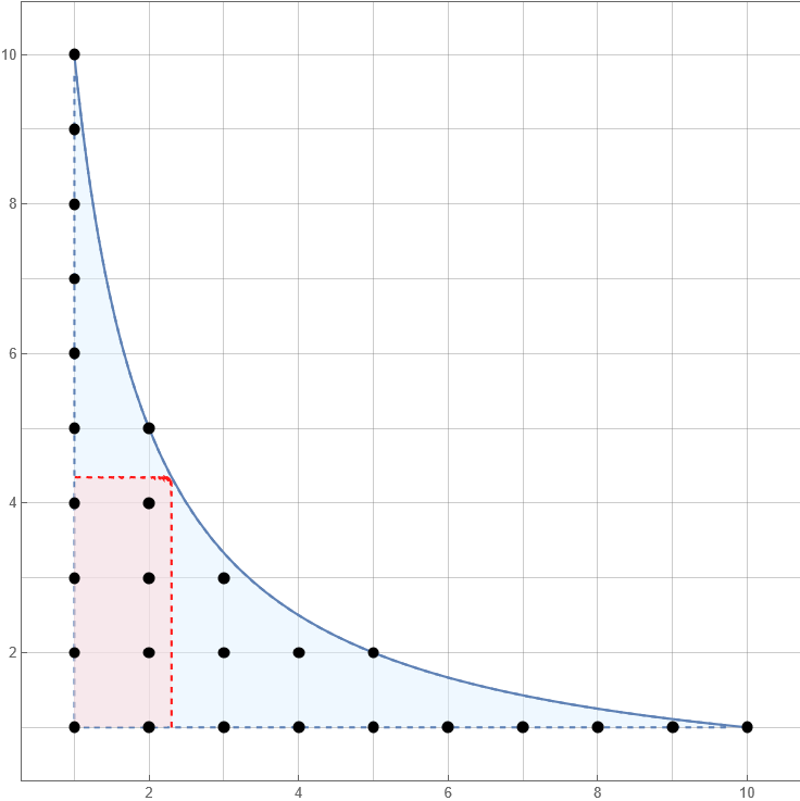
Here we have $x = 10$, $\alpha = 2.3$ and $\beta = x/\alpha \approx 4.3$.
The black points are those $(a, b)$ for which we have a term $f(a)g(b)$ in the sum.
The first term $\sum_{a \leq \alpha} f(a)G(x/a)$ in the sum computes the sum over all the points $(a, b)$ in the left section (all points for which $a \leq \alpha$). The second term likewise computes the sum over all the points in the lower section, for which $b \leq \beta$. The red highlighted rectangle is summed by $F(\alpha)G(\beta)$, and it is the set of points we have added to the sum twice.
This idea was also used in my post about the Lucy_Hedgehog algorithm. We will usually pick $\alpha = \beta = \sqrt{x}$ but sometimes it helps to be able to balance the break point based on how hard $f$ and $g$ are to sum individually. Let’s see what happens for $u*u = d$.
In this case, we have $F(x) = G(x) = \lfloor x \rfloor$, so pick $\alpha = \beta = \sqrt{x}$.
\[\begin{align*} \sum_{n \leq x} d(n) &= \sum_{n \leq \sqrt{x}} u(n) \left \lfloor \frac{x}{n} \right \rfloor + \sum_{n \leq \sqrt{x}} \left \lfloor \frac{x}{n} \right \rfloor u(n) - \left \lfloor \sqrt{x} \right \rfloor^2\\ &= 2\sum_{n \leq \sqrt{x}} \left \lfloor \frac{x}{n} \right \rfloor - \left \lfloor \sqrt{x} \right \rfloor^2 \end{align*}\]Immediately we have an algorithm to compute $D(x)$ in $O(\sqrt{x})$ time! Here it is in Nim.
proc divisorSummatory(x: int64): int64 =
  ##Computes d(1) + ... + d(x) in O(x^(1/2)) time.
  var xsqrt = isqrt(x)
  for n in 1..xsqrt:
    result += 2*(x div n)
  result -= xsqrt*xsqrt
For $D(x)$, it’s possible to do it in something like $O(x^{1/3})$ time, but I’ll cover that in a later post because it’s much more complicated and uses a very different technique.
So with this, if we’re able to sum $f$ and $g$ in a reasonable amount of time, we’re able to sum $f*g$ as well. This will be a crucial feature of the more complex methods.
Tangent: Linear Sieving
In the future we’re going to use what I think are generally referred to as “sieving techniques” to compute all values of given arithmetic functions $f(n)$ over short intervals $n \leq y$.
Let’s try doing this for the function $f(n) = d(n)$.
As before, we’ll be smart, iterating over the potential divisors $k$ of $n$ and then noting that the integers $n$ divisible by $k$ are simply $k, 2k, 3k$, etc.
var d = newSeq[int](y+1)
for k in 1..y:
  #increment d[k*j] for all multiples k*j <= y
  for j in 1..(y div k):
    inc d[k*j]
Now this runs in about $O\left(\sum_{k \leq y} \frac{y}{k}\right) = O\left(y \log y\right)$ time, which is just barely above linear.
For most purposes this will be perfectly fine.
Let’s take a look at how it looks if we do a very basic sieve for $\varphi$.
The idea here is to exploit the multiplicativity of $\varphi$.
If $p$ is a prime not dividing $m$, then $\varphi(m p^e) = \varphi(m) p^{e-1}(p-1)$.
From this we obtain the formula we’ll use, $\varphi(n) = n \prod_{p \mid n} \frac{p-1}{p}$.
So what we’re going to do is initialize phi[n] = n for all n, and then fix the contribution of each prime factor separately.
To recognize when we have a prime, we’re going to check whether phi[n] has been modified yet. We can just check if phi[p] == p - if it is, p is a prime, and we fix the contributions of p.
var phi = newSeq[int](y+1)
for k in 1..y: phi[k] = k
#initialized
for p in 2..y:
  if phi[p] == p:
    for k in 1..(y div p):
      phi[p*k] = (phi[p*k] div p) * (p-1)
Nice and easy! This now takes $O\left(\sum_{p \leq y} \frac{y}{p}\right)$ time, which is $O\left(y \log \log y\right)$, so slightly faster than the basic one for the divisor function. Generally those functions that only need their prime factor contributions fixed can be done in this way.
Along this line of thinking, for basically any multiplicative function, we can do this calculation in a flat $O(y)$ time. This generally offers a good speedup to the summation methods I’ll be detailing later. The best explanation I’ve found on this is in this CodeForces blog post by Nisiyama_Suzune. I am going to refrain from explaining how it works in depth because the implementation of this subroutine doesn’t intersect the implementation of the later methods much at all. That is, I can use this as a black box which we will just avoid looking at for too long. Read that post! Here’s code I’ll be using to produce the values of $f\ast u$ given the values of $f$ in linear time, using an extra $O(y)$ space. It could be easily modified to produce the values of $f\ast g$ given any multiplicative $f, g$.
proc linearSieveProdUnit(f: seq[int64], m: int64): seq[int64] =
  #Returns the dirichlet product of f and u in linear time.
  #Assumes f[1] = 1 and that f is multiplicative.
  #m is modulus.
  #linear sieves - https://codeforces.com/blog/entry/54090
  let y = f.len
  newSeq(result, y)
  var composite: seq[bool]
  var pow = newSeq[int](y) #power of leastprimefactor(n) in n
  newSeq(composite, y)
  var prime = newSeq[int]()
  result[1] = 1
  for i in 2..<y:
    if not composite[i]:
      prime.add i
      result[i] = f[i] + 1 #i is prime
      pow[i] = i
    for j in 0..<prime.len:
      if i*prime[j]>=y: break
      composite[i*prime[j]] = true
      if i mod prime[j] == 0:
        pow[i*prime[j]] = pow[i] * prime[j]
        var v = i div pow[i]
        if v != 1:
          result[i*prime[j]] = (result[v] * result[prime[j] * pow[i]]) mod m
        else:
          var coef = 0'i64
          var A = 1
          var B = pow[i] * prime[j]
          while B > 0:
            coef += f[A]
            coef = coef mod m
            A *= prime[j]
            B = B div prime[j]
          result[i*prime[j]] = coef
        break
      else:
        result[i*prime[j]] = result[i]*result[prime[j]]
        pow[i*prime[j]] = prime[j]
Summing Generalized Divisor Functions
This section is about a function we haven’t yet seen. Here’s how it’s defined.
The generalized divisor function $d_k(n)$ is the number of ways to write $n$ as a product of $k$ naturals. It’s the function with the Dirichlet series $\zeta(s)^k$.
In other words, $d_1(n) = u(n) = 1$ for all $n$, and $d_k = u * d_{k-1}$, so $d_k(n) = \sum_{a \mid n} d_{k-1}(a)$.
Clearly $d_1(n) = u(n) = 1$ for all $n$, since there is only one way to write $n$ as the product of only a single integer. For $d_2(n)$, we’re counting the representations $n = ab$, and since $b$ is determined completely by $n$ and $a$, this is just the number of divisors of $n$. That is, $d_2(n) = d(n)$. In the previous section we figured out how to sum this quickly, but how about.. $d_5$ for example?
If we attempted to just use the hyperbola method over and over again with no modifications we would get worse and worse runtime, as follows.
We know $d_1$ can be summed in constant time, and that $d_2$ can be summed in $O(x^{1/2})$ time.
How about $d_3$?
Brainlessly apply the hyperbola method. We obtain
\[D_3(x) = \sum_{n \leq x} d_3(n) = \sum_{n \leq \alpha} D_2\left(\frac{x}{n}\right) + \sum_{n \leq \beta} d_2(n) \left\lfloor \frac{x}{n}\right\rfloor - \left\lfloor\alpha\right\rfloor D_2(\beta)\]The last term takes $O(\beta^{1/2})$ time of course. The first one takes $O\left(\sqrt{x\cdot\alpha}\right)$ time, and the second takes $O(\beta)$ time if we sieve $d_2$ in linear time. If we optimize $\alpha$ and $\beta$ we choose $\alpha = x^{1/3}$ and $\beta = x^{2/3}$, for a total runtime of $O(x^{2/3})$.
If we repeat this for $D_4$ you’ll end up choosing $\alpha = x^{1/4}$ and $\beta = x^{3/4}$ for a total runtime of $O(x^{3/4})$.
Also notice that we also require $O(x^{3/4})$ space for this, which is getting pretty large.
By induction, we can compute $D_k(x)$ in $O(x^{1 - 1/k})$ time, which as $k$ gets large is probably even worse than linear just due to a growing constant factor which I’ve ignored. Here we’re going to show how we can cap the runtime to $O(k x^{2/3})$ while using $O(x^{2/3})$ space.
The key idea here is again essentially from my last post.
We’re going to pick some $\sqrt{x} \leq y \leq x$ to be specified later and compute $D_k(v)$ for the key values $v \leq y$ by linear sieving, which will take $O(y)$ time. The rest of them will be done using the hyperbola method, using $\alpha = \beta = \sqrt{x}$. Here’s a slightly more specific layout of the ideas:
Algorithm (Computing $D_k$(x) Iteratively)
\[D_j(v) = \sum_{n \leq \sqrt{v}} D_{j-1}\left(\frac{v}{n}\right) + \sum_{n \leq \sqrt{v}} d_{j-1}(n) \left \lfloor \frac{v}{n} \right \rfloor - D_{j-1}(\sqrt{v})\left\lfloor\sqrt{v}\right\rfloor\]
- Set $y \propto x^{2/3}$.
Set an arraysmallof length $y$ to store $D_1(k)$ for $k \leq y$.
Set an arraybigof length $x/y$ to store $D_1(x / k)$ for $k < x/y$.- For $j$ from $2$ to $k$, we’ll update our arrays to reflect $D_j$ instead:
2a. Updatebigvalues first, then updatesmallvalues by sieving in $O(y)$.
Thebigvalues can be updated by the formula
How much time do we dedicate to updating the big array? It takes
\[O\left(\sum_{k < x/y} \sqrt{x/k}\right) = O\left(\int_1^{x/y} \sqrt{\frac{x}{k}}dk \right) = O\left(x/\sqrt{y}\right)\]If we want to minimize the total time to update both arrays, $O\left(y + x/\sqrt{y}\right)$, we need to pick $y$ to be on the order of $x^{2/3}$. The resulting time (and space) complexity is $O\left(x^{2/3}\right)$. Since we have to update it $k$ times, the runtime is $O\left(kx^{2/3}\right)$ in the end!1
You’ll have to poke at the constant coefficient on $y$ in your implementation.
Very short note here - I’m reusing the FIArray container from last time. Read the relevant section of the linked post if you want some context, but here it’s just an easy container for our data. The following is an implementation of this algorithm.
proc genDivisorSummatory(x: int64, k: int, m: int64): FIArray =
  ##Computes d_k(1) + ... + d_k(x) mod m in O(k x^(2/3)) time.
  var y = (0.55*pow(x.float, 2.0/3.0)).int64
  y = max(y, isqrt(x))
  var small = newSeq[int64](y+1)
  var big = newSeq[int64]((x div y) + 1)
  #initialize them to D_1, sum of u(n) = 1
  for i in 1..y: small[i] = i mod m
  for i in 1..(x div y): big[i] = (x div i) mod m
  #iteration time!
  for j in 2..k:
    #update big first
    for i in 1..(x div y):
      let v = x div i
      let vsqrt = isqrt(v)
      var bigNew = 0'i64
      for n in 1..vsqrt:
        #add D_{j-1}(v/n) = D_{j-1}(x/(i*n))
        if v div n <= y: bigNew += small[v div n]
        else: bigNew += big[i*n]
        #add d_{j-1}(n) floor(v/n)
        #to do so, grab d_{j-1}(n) from small = sum d_{j-1}
        bigNew += (small[n] - small[n-1]) * (v div n)
        bigNew = bigNew mod m
      bigNew -= small[vsqrt]*vsqrt
      big[i] = bigNew mod m
    #update small using sieving
    #be lazy...
    #convert small from summation to just d_{j-1}, convolve, then convert back
    for i in countdown(y, 1):
      small[i] -= small[i-1]
    small = linearSieveProdUnit(small, m)
    for i in 1..y:
      small[i] = (small[i] + small[i-1]) mod m
  #shove them all into an FIArray for easy use
  var Dk = newFIArray(x)
  for v in Dk.keysInc:
    if v <= y: Dk[v] = small[v]
    else: Dk[v] = big[x div v]
  return Dk
The important thing to learn from this section is that, when we’re dealing with summations of multiplicative functions, we should probably store sieved values up to about $x^{2/3}$ and then the sums up to larger $\lfloor x/k \rfloor$. If we have this data for two functions $f$ and $g$, then we can spend $O(x^{2/3})$ time to generate the same data for $f*g$.
Summing $\mu$ and $\varphi$
First notice that $\varphi = \mu * N$ so that if we can sum $\mu$, we can also sum $\varphi$.
The summatory function of $\mu$ is called the Mertens function. It’s been studied in detail by a lot of people because it’s a very important function. We write it as $M(x) = \sum_{n \leq x} \mu(n)$. The prime number theorem is equivalent to $M(x)/x \to 0$ as $x$ goes to infinity (read Apostol’s book if you want to see why).
Computing $M(x)$ in Sublinear Time
The key idea here is again similar to the one in my post about prime counting, in that we’ll use the “square root trick” again.
Let’s start with the formula $\mu*u = I$, which when plugged into the hyperbola method gives the following for all $v \geq 1$:
\[\sum_{n \leq \sqrt{v}} \mu(n)\left \lfloor \frac{v}{n}\right\rfloor + \sum_{n \leq \sqrt{v}} M\left(\frac{v}{n}\right) - \lfloor \sqrt{v} \rfloor M\left(\sqrt{v}\right) = 1\]We can suppose we’ve sieved at least the first $\sqrt{x}$ values of $\mu$. Let’s also assume we’ve computed $M\left(\frac{x}{n}\right)$ for $n > 1$. Then we’d have
\[M(x) = 1 - \sum_{n \leq \sqrt{x}} \mu(n)\left \lfloor \frac{x}{n}\right\rfloor - \sum_{2 \leq n \leq \sqrt{x}} M\left(\frac{x}{n}\right) + \lfloor \sqrt{x} \rfloor M\left(\sqrt{x}\right)\]Notice that if we plug in $x = 1$ we get $M(x)$ again in the right hand side, so we should just set $M(1) = 1$ manually to avoid issues.
Then if we know the values of $M(x/n)$ for $n > 1$, we can compute $M(x)$ in $O(\sqrt{x})$ time.
This sort of structure is going to be very similar for a lot of the functions we’ll sum, so again we’re going to be using the old FIArray as a container here.
The algorithm for computing $M(x)$ will proceed as follows:
Algorithm (Mertens in $O(x^{3/4})$)
\[M(v) = 1 - \sum_{n \leq \sqrt{v}} \mu(n)\left\lfloor \frac{v}{n}\right\rfloor - \sum_{2 \leq n \leq \sqrt{v}} M\left(\frac{v}{n}\right) + \lfloor \sqrt{v} \rfloor M\left(\sqrt{v}\right)\]
- Sieve $\mu(n)$ for $n \leq \sqrt{x}$.
- For each key value $v$ in increasing order, set
The first step takes $O(\sqrt{x})$ time. How about the rest?
The lower key values take a total time of
\[O\left(\sum_{v \leq \sqrt{x}} \sqrt{v}\right) = O\left(\sqrt{x} \sqrt{\sqrt{x}}\right) = O\left(x^{3/4}\right)\]The upper key values $v = \lfloor x/k \rfloor$ for $k < \sqrt{x}$ contribute
\[O\left(\sum_{k \leq \sqrt{x}} \sqrt{\frac{x}{k}}\right) = O\left(\int_1^{\sqrt{x}} \sqrt{\frac{x}{k}}dk\right) = O\left(x^{3/4}\right)\]So this easy algorithm only takes $O(x^{3/4})$ time and $O(x^{1/2})$ space.
Here’s an implementation:
proc mertens(x: int64): FIarray =
  ##Computes mu(1) + ... + mu(x) in O(x^(3/4)) time.
  var M = newFIArray(x)
  var mu = mobius(x.isqrt.int+1)
  for v in M.keysInc:
    if v == 1:
      M[v] = 1
      continue
    var muV = 1'i64
    var vsqrt = isqrt(v)
    for i in 1..vsqrt:
      muV -= mu[i]*(v div i)
      muV -= M[v div i]
    muV += M[vsqrt]*vsqrt
    M[v] = muV
  return M
This takes 7 seconds to compute $M(10^{12}) = 62366$ on my laptop, which is pretty good!
The way we make this faster is yet again very similar to how we made the Lucy_Hedgehog prime counting algorithm faster in the last post - read it if you haven’t yet!
We’re going to do the same thing as for our generalized divisor function sums, and pick some $\sqrt{x} \leq y \leq x$ to be specified later. We will compute $M(v)$ for the key values $v \leq y$ by sieving, which will take $O(y)$ time. The rest of them will be done in the way described previously.
How much time do the remaining key values $v = \lfloor x/k \rfloor > y$ take?
\[O\left(\sum_{k < x/y} \sqrt{\frac xk}\right) = O\left(\int_1^{x/y} \sqrt{\frac xk}dk \right) = O\left(\frac x{\sqrt{y}}\right)\]If we want to minimize the total time $O\left(y + x/\sqrt{y}\right)$, we need to pick $y$ to be on the order of $x^{2/3}$. The resulting time (and space) complexity is $O\left(x^{2/3}\right)$ which is better.
In your implementation, you should try different constants to see which one looks like it works the best. For me, choosing $y = 0.25x^{2/3}$ looked alright. You should also cap it by some limit based on how much memory you have available.
Algorithm (Mertens in $O(x^{2/3})$)
\[M(v) = 1 - \sum_{n \leq \sqrt{v}} \mu(n)\left\lfloor \frac{v}{n}\right\rfloor - \sum_{2 \leq n \leq \sqrt{v}} M\left(\frac{v}{n}\right) + \lfloor \sqrt{v} \rfloor M\left(\sqrt{v}\right)\]
- Pick $y$ on the order of $x^{2/3}$.
- Sieve $\mu(n)$ for $n \leq y$.
- Accumulate this array, so that you store $M(v)$ for all $v \leq y$.
The value $\mu(v)$ can be recovered by $M(v) - M(v-1)$ when needed.- For each key value $v > y$ in increasing order, set
Here’s how this could look in Nim:
proc mertensFast(x: int64): FIarray =
  ##Computes mu(1) + ... + mu(x) in O(x^(2/3)) time.
  var M = newFIArray(x)
  var y = (0.25*pow(x.float, 2.0/3.0)).int
  y = min(y, 1e8.int) #adjust this based on how much memory you have
  var smallM = mobius(y+1)
  #we're actually going to store mu(1) + ... + mu(k) instead
  #so accumulate
  for i in 2..y: smallM[i] += smallM[i-1]
  #now smallM[i] = mu(1) + ... + mu(i)
  for v in M.keysInc:
    if v <= y:
      M[v] = smallM[v]
      continue
    var muV = 1'i64
    var vsqrt = isqrt(v)
    for i in 1..vsqrt:
      muV -= (smallM[i] - smallM[i-1])*(v div i)
      muV -= M[v div i] #M[v div 1] is initialized to zero in Nim.
    muV += M[vsqrt]*vsqrt
    M[v] = muV
  return M
Now we get $M(10^{12})$ in less than 2 seconds on my laptop!
Doing It For $\varphi$?
Before, we computed the Mertens function without calling notice to its size - generally it’s very small. In the case of the totient summatory function $\Phi(x) = \sum_{n \leq x} \varphi(x)$, it will be quite large. To calculate it then, I’ll include a modulus m in the functions. If you are using Python or something where you don’t have to worry about overflows, then there’s no real need for that aside from memory concerns.
Like I said before though, we can compute the totient summatory function $\Phi(x)$ in $O(\sqrt{x})$ further time by using the hyperbola theorem (using $\varphi = \mu * N$) as follows:
proc sumN(x: int64, m: int64): int64 =
  ##Sum of n from 1 to x, mod m.
  var x = x mod (2*m) #avoid overflows
  if x mod 2 == 0:
    return ((x div 2) * (x+1)) mod m
  else:
    return (((x+1) div 2) * x) mod m

proc totientSummatoryFast1(x: int64, m: int64): int64 =
  ##Computes Phi(x) mod m in O(x^(2/3)) time.
  ##Does NOT compute any other Phi(x/n).
  var M = mertensFast(x)
  #phi = mu * N
  var xsqrt = M.isqrt
  for n in 1..xsqrt:
    result += (M[n] - M[n-1]) * sumN(x div n, m)
    result = result mod m
    result += n * M[x div n]
    result = result mod m
  result -= sumN(xsqrt, m)*M[xsqrt]
  result = result mod m
  if result < 0: result += m #this can happen
And just like that we have the totient summatory function in $O(x^{2/3})$ time.
It computes $\Phi(10^{12}) \equiv 804025910 \bmod 10^9$ in about 2.9 seconds on my laptop.
Alternatively, we could apply the logic from our Mertens function directly, by using the relation $\varphi * u = N$ and the exact same partial-sieving trick as before. Here’s how that looks:
proc totientSummatoryFast2(x: int64, m: int64): FIarray =
  ##Computes phi(1) + ... + phi(x) mod m in O(x^(2/3)) time.
  var Phi = newFIArray(x)
  var y = (0.5*pow(x.float, 2.0/3.0)).int
  y = min(y, 1e8.int) #adjust this based on how much memory you have
  var smallPhi = totient[int64](y+1)
  #again store phi(1) + ... + phi(k) instead
  #so accumulate
  for i in 2..y:
    smallPhi[i] = (smallPhi[i] + smallPhi[i-1]) mod m
  #now smallPhi[i] = phi(1) + ... + phi(i)
  for v in Phi.keysInc:
    if v <= y:
      Phi[v] = smallPhi[v]
      continue
    var phiV = sumN(v, m)
    var vsqrt = isqrt(v)
    for i in 1..vsqrt:
      phiV -= ((smallPhi[i] - smallPhi[i-1])*(v div i)) mod m
      phiV -= Phi[v div i]
      phiV = phiV mod m
    phiV += Phi[vsqrt]*vsqrt
    phiV = phiV mod m
    if phiV < 0: phiV += m
    Phi[v] = phiV
  return Phi
This runs barely slower than the method to compute a single $\Phi(x)$ from the Mertens values - probably it’s just easier to store the Mertens values because they’re so small.
It computes $\Phi(10^{12})$ in about 3.5 seconds.
So, this previous method will work nicely whenever we want to sum a function $f$ such that we have easily summable functions $g, h$ with $f*g = h$, and such that $f$ can be sieved in linear (or approximately linear) time. This is a very wide selection of functions, but there are others yet we can’t deal with.
Powerful Numbers Trick
This is perhaps a more specialized technique.
Suppose we want to sum the multiplicative function $f(n)$, and we have an easily summable multiplicative function $g(n)$ so that $f(n) = g(n)$ for any squarefree $n$.
It’s sufficient that $f(p) = g(p)$ for primes.
I like to think of this as an approximation of $f$ to first prime order. The choice of $g$ is probably very subjective, and some ingenuity may be required to find the perfect choice. In general if $f(p)$ is simple, the choice for $g$ will be obvious.
Whenever we have such a situation, the function $f/g = h$ (division being in terms of Dirichlet inverses) will have the nice property that $h(n) = 0$ for all $n$ that are not “powerful”.
By “powerful”, I mean that if a prime $p$ divides $n$, then $p^2$ also divides $n$.
So for example $2^3 5^2$ is powerful, but $2^7 5^1 7^3$ is not powerful. As it turns out, there are vanishingly many powerful integers up to $x$, actually $O(\sqrt{x})$ of them (see this Wikipedia article).
Why is $h(n) = 0$ for non-powerful integers $n$?
Suppose $p$ divides $n$ and $p^2$ does not. Then if $n = pk$, we have $h(n) = h(pk) = h(p)h(k)$. But since $h*g=f$, we have $h(p)g(1) + h(1)g(p) = f(p)$, so that $h(p) + g(p) = f(p)$. Then since $f(p) = g(p)$ we have to have $h(p) = 0$, so that $h(n) = 0$ as well.
So think of $h$ as a correction to $f$. The fact that $h(n)$ is usually zero reflects that $g$ is a pretty decent approximation to $f$, only really needing to be nudged at very highly composite $n$.
Then since $f = g*h$, we have $F(x) = \sum_{n \leq x} h(n)G(x/n)$ over powerful $n \leq x$. Since $h$ is also multiplicative, you can generate the powerful numbers along with their corresponding values of $h$, making this a pretty fast summation algorithm.
Our example here will be summing $f(n) = d(n^2)$.
Let’s see how it looks at primes.. $f(p) = d(p^2) = 3$. What function do we know of, which we can already sum relatively quickly, such that $g(p) = 3$?
One may have the creative insight that $3 = 1+1+1$ and come to the conclusion that setting $g(n) = d_3(n)$ is a good idea. We know from the generalized divisor function section that we can sum this in $O(x^{2/3})$ time if we’re careful, which is not so bad.
As a reminder we’ll write $D_3(x)$ for the sum of $d_3(n)$ over $n \leq x$.
Now let’s find out what sort of function $h = f / d_3$ is.
Bell Series
Given a multiplicative function $f(n)$, the Bell series of $f$ given a prime $p$ is the formal power series
\[f_p(z) = \sum_{e \geq 0} f(p^e) z^e\]You can read about these in Apostol’s book. A helpful feature is that
\[(f*g)_p(z) = f_p(z) g_p(z)\]Therefore if we want to compute the closed form of $h = f/d_3$ at prime powers we can divide the Bell series for $f$ and $d_3$ and use the power series for the result.
We compute
\[\begin{align*} f_p(z) &= \sum_{e \geq 0} (2e+1)z^e\\ (d_3)_p(z) &= \sum_{e \geq 0} \binom{e+2}{e} z^e\\ &= (u\ast u\ast u)_p(z) = \left(\sum_{e \geq 0} z^e\right)^3\\ h_p(z) &= \frac{\sum_{e \geq 0} (2e+1)z^e}{\left(\sum_{e \geq 0} z^e\right)^3}\\ &= \frac{(1-z)^3(1+z)}{(1-z)^2} = (1-z)(1+z) = 1-z^2 \end{align*}\]So we know $h(p) = 0$, $h(p^2) = -1$, and $h(p^e) = 0$ for $e > 2$.
You can see that $h(n^2) = \mu(n)$, so we’re actually quite lucky in this case, and we can now write
We can simply compute $D_3(v)$ for all key values $v$, sieve $\mu$ up to $\sqrt{x}$, and compute the sum. The total runtime is $O(x^{2/3})$, and it looks like this:
proc sumDn2(x: int64, m: int64): int64 =
  ##Computes d(1^2) + d(2^2) + d(3^2) + ... + d(x^2) in O(x^(2/3)) time.
  var D3 = genDivisorSummatory(x, 3, m)
  var xsqrt = D3.isqrt.int #isqrt(x)
  var mu = mobius(xsqrt+1)
  for n in 1..xsqrt:
    result += mu[n]*D3[x div (n*n)]
    result = result mod m
  if result < 0: result += m
  return result
This takes about 8s to compute $\sum_{n \leq 10^{12}} d(n^2)$ on my laptop.
We got lucky here in that $h = f/g$ was zero even more often than we’d expect it to be.
Let’s try a case which does not work out quite that way.
Suppose we define $f(n)$ to be the largest powerful divisor of $n$. In other words, $f$ is the multiplicative function with $f(p) = 1$ and $f(p^e) = p^e$ for $e > 1$.
Clearly here we’ll choose $g(n) = u(n) = 1$ for all $n$, and then $h = f/g$ has $h(p) = 0$, $h(p^2) = p^2 - 1$, and $h(p^e) = p^e - p^{e-1}$ for $e > 2$.
Now, when it comes to generating all the powerful $n \leq x$ along with their values $h(p^e)$, I think a common approach I’ve seen (I think from baihacker) is to just do a recursive depth first search, adding prime factors in order. We’ll do something similar but with a stack.
In the following, $h(p^e)$ is represented by a two variable function h(p, e: int64): int64.
I’ll also include a modulus. You can also implement a version without a modulus for when you know values are going to be small which will save a little bit of time.
Algorithm (Powerful Numbers Iterator)
- Start by noting that no prime greater than $\sqrt{x}$ can divide any powerful number up to $x$. So compute the primes up to $\sqrt{x}$ using a simple Eratosthenes sieve into a list, say
ps.- Initialize a stack
stkwhich contains tuples(n, hn, i), wherehnis the value $h(n)$, andiis the index of the next prime to consider in the list.
This stack should start with containing(1, 1, 0).- If the stack is empty we are finished.
If the stack is nonempty, pop(n, hn, i)from the stack.- If
i == ps.len, then we’ve already considered adding all prime factors ton, so we should just yield(n, hn)and return to step 3.
Setp = ps[i]as anint64.
Ifn*p*p > x, we will never be adding any more prime factors ton, so we should yield again(n, hn)and return to step 3. To avoid overflow errors here, check ifp*p > x div ninstead.- If we’ve gotten here, there’s the possibility of adding a larger prime factor to
n. For the case that we don’t add a factor ofp, we push(n, hn, i+1)to the stack.
In the other case, we’ll be adding a factor of (at least)p*p.
Initializepp = p*pfor the power ofpwe’re factoring inton, and sete = 2to track the current power ofpwe’re considering.
Whilen*pp <= x(rather checkpp <= x div n), push(n*pp, (hn*h(p,e)) mod m, i+1)to the stack to be considered later. Be careful about possible overflows inpphere, so before doingpp *= pande += 1be sure to make sure it won’t be too big.
One way to check this is by testingpp > (x div n) div p, if this is true then it’ll be too big and we can just break.
Once finished adding factors ofpton, return to step3.
iterator powerfulExt(x: int64, h: proc (p, e: int64): int64, m: int64): (int64, int64) =
  ##Yields (n, h(n) mod m) where n are the O(sqrt x) powerful numbers
  ##up to x, and h is any multiplicative function.
  var nrt = isqrt(x).int
  var res = @[(1'i64, 1'i64, 0)]
  var ps = eratosthenes(nrt+1)
  while res.len > 0:
    var (n, hn, i) = res.pop
    var p: int64
    if i < ps.len: p = ps[i]
    if i >= ps.len or p*p > x div n:
      #note: value of p is only used here if i < ps.len
      yield (n, hn)
      continue
    res.add (n, hn, i+1)
    var pp = p*p
    var e = 2
    while pp <= x div n:
      res.add (n*pp, (hn*h(p, e)) mod m, i+1)
      if pp > (x div n) div p: break
      pp *= p
      e += 1
So now when we want to use our powerful numbers trick we can call on this.
In our case, the remaining work is easy:
proc sumPowerfulPart(x: int64, m: int64): int64 =
  ##Sums the function f(p) = 1 and f(p^e) = p^e for e > 1.
  #make function h to pass forward
  proc h(p, e: int64): int64 =
    if e == 0: return 1
    if e == 1: return 0
    if e == 2: return (p*p - 1) mod m
    return (powMod(p, e, m) - powMod(p, e-1, m) + m) mod m
  for (n, hn) in powerfulExt(x, h, m):
    result += hn * ((x div n) mod m)
    result = result mod m
  return result
Here, x div n is the summatory function of $g(n) = 1$ up to $x/n$. This can sum up to $10^{15}$ in about 3s on my laptop, and uses a very modest amount of memory.
When $G(x)$ can be computed in exactly $O(\sqrt{x})$ time, the runtime for $F(x)$ will be $O(\sqrt{x} \log(x))$. If $G(x)$ can be computed faster, then iterating on the powerful numbers will dominate the runtime and it’ll be $O(\sqrt{x})$. When $G(x)$ is slower, then the runtime of $F(x)$ will basically match that of $G(x)$.
Note on Picking $g$
It helps, here, to be well versed on the values of many multiplicative functions at primes.
Here’s a table.
| Function $g$ | Value $g(p)$ |
|---|---|
| $N$ | $p$ |
| $u$ | $1$ |
| $\mu$ | $-1$ |
| $\varphi = N*\mu$ | $p-1$ |
| $d=u*u$ | $2$ |
| $d_k$ | $k$ |
| $\sigma_\alpha$ | $p^\alpha+1$ |
One pattern that is evident from definitions is that $(f*g)(p) = f(p) + g(p)$. So if we desire some form for $g(p)$ and we can break it up into a sum of ones that we know, we can just use the Dirichlet convolution of those parts.
For example, if we wanted to sum a function with $f(p) = 2p+1$, we could write $2p+1 = p + (p+1)$ and choose $g = N * \sigma_1$. Luckily enough, both $N$ and $\sigma_1$ are feasibly summable using the techniques we’ve already explored. Thus with the powerful numbers trick we can manage this kind of function too!
Tangent: How Not To Count Primes
In my prime counting post we developed an algorithm to compute $\pi(x)$, the number of primes up to $x$, in something like $O(x^{2/3} (\log x \log \log x)^{1/3})$ time using Fenwick trees and Lucy’s algorithm.
This time we’re going to be doing something no one should actually do, and use sums of multiplicative functions to develop an algorithm to compute $\pi(x)$ in $O(x^{2/3} \log(x))$ time. Really, it’s not actually so bad asymptotically, but it is worse. Don’t use this.
The setup here will rely on the following functions:
\[\begin{align*} f_k(n) &:= k^{\Omega(n)}\\ F_k(x) &:= \sum_{n \leq x} f_k(n) \end{align*}\]Here, $\Omega(n)$ is the number of prime factors of $n$ with multiplicity.
First, notice that $\Omega(n) + \Omega(m) = \Omega(nm)$, so that $f_k(n)f_k(m) = f_k(nm)$, and $f_k$ is not only multiplicative, but completely multiplicative.
Okay, so let’s suppose we can compute every $F_k(x)$ that we wish. How do we get $\pi(x)$?
That this is possible was first noted, I think, by Project Euler user asaelr.
Suppose we group the integers $n$ up to $x$ based on the value of $\Omega(n)$. We have
\[\begin{align*} F_k(x) &= \sum_{e \geq 0} \sum_{\substack{n \leq x \\ \Omega(n) = e}} k^e\\ &= \sum_{e \geq 0} k^e \pi_e(x) \end{align*}\]Here I’m writing $\pi_e(x)$ for the number of integers up to $x$ with exactly $e$ prime factors.
Clearly since the integer with the most prime factors up to $x$ is just $2^{\lfloor \log_2(x) \rfloor}$, we only actually need to consider the terms in the sum with $e \leq \log_2(x)$.2 Then it becomes clear that, if $x$ is fixed, the function $F_k(x)$ is actually a polynomial in $k$ of degree $\lfloor \log_2(x) \rfloor$, and the linear coefficient is $\pi(x)$.
The strategy then is to compute about $\log_2(x)+1$ values of $F_k(x)$ and then to use polynomial interpolation to solve for the missing coefficients. The interpolation takes negligible time.
Let’s try to use the Powerful Numbers Trick here and examine the form of $f_k(p)$.
Clearly it’s $f_k(p) = k$, and so the best option we have for $g$ is $d_k$, which we have figured out how to sum in $O(x^{2/3})$ time. Moreover though, our algorithm already goes through all $k$ up to some limit, so all we have to do is, at each step, use the trick to compute $F_k(x)$ and save it to an array.
What does $h_k = f_k / d_k$ look like? Not very nice unfortunately.
The Bell series is
\[(h_k)_p(z) = \frac{\sum_{e \geq 0} k^e z^e}{\left(\sum_{e \geq 0} z^e\right)^k} = \frac{(1-z)^k}{1-kz}\]From this, the Binomial theorem, and looking at the generating function,
\[h_k(p^e) = \sum_{i=0}^e \binom{k}{i}(-1)^i k^{e-i}\]Thankfully for us, this doesn’t depend on $p$, so one option is to compute a small table of binomial coefficients and then values of $h_k(p^e)$ in time $O(\log(x)^2)$ or something.
One other option that I think works fine, especially if $h_k(p^e)$ does depend on $p$, or even if you want to build a fully generic implementation of this idea, is to create a memoized recursive function.
If you want to get the values of $h = f/g$, you could just use
\[\begin{align*} (h*g)(p^e) &= f(p^e)\\ \sum_{i=0}^e h(p^i)g(p^{e-i}) &= f(p^e)\\ h(p^e) + \sum_{i=0}^{e-1} h(p^i)g(p^{e-i}) &= f(p^e)\\ h(p^e) &= f(p^e) - \sum_{i=0}^{e-1} h(p^i)g(p^{e-i}) \end{align*}\]I don’t really care to do a runtime analysis on this technique but it seems fine.
Anyways, I’m going to choose the binomial expression mentioned earlier because it’s more straightforward in this case. Do what you want depending on your situation.
The last step here, given the values of a polynomial, is to interpolate the coefficients mod $m$. This is something that’s honestly a little annoying to do, but we only need the linear coefficient. To get that we can basically modify Neville’s algorithm a little bit as follows:
proc linearCoefficient(inputs, outputs: seq[int64], m: int64): int64 =
  var p0 = outputs
  var p1 = newSeq[int64](inputs.len)
  #(refer to wikipedia)
  #here, p0[j] stores the constant coefficient of p_{j,j}(x)
  #and p1[j] stores the linear coefficient
  for i in 1..inputs.high:
    #now we will make p0[j] and p1[j] refer to p_{j,i+j}(x)
    for j in 0..inputs.high - i:
      p0[j] = (inputs[j]*p0[j+1]-inputs[j+i]*p0[j]) mod m
      p0[j] = (p0[j]*modInv(m - inputs[j+i] + inputs[j], m)) mod m
      p1[j] = (p0[j] - inputs[j+i]*p1[j] - p0[j+1] + inputs[j]*p1[j+1]) mod m
      p1[j] = (p1[j]*modInv(m - inputs[j+i] + inputs[j], m)) mod m
  return p1[0]
This isn’t what I’m here to talk about though so we’re going to move on.
Here’s how the algorithm looks, put together:
proc primePi(x: int64, m: int64): int64 =
  ##Computes pi(x) mod m in O(x^(2/3) log x) time.
  ##See genDivisorSummatory.

  var y = (0.55*pow(x.float, 2.0/3.0)).int64
  y = max(y, isqrt(x))
  var small = newSeq[int64](y+1)
  var big = newSeq[int64]((x div y) + 1)
  #initialize them to D_1, sum of u(n) = 1
  for i in 1..y: small[i] = i mod m
  for i in 1..(x div y): big[i] = (x div i) mod m

  var k = 1
  while (1'i64 shl (k+1)) <= x: inc k
  #we need F_j(x) for j from 0 to k
  var F = newSeq[int64](k+1)
  F[0] = 1
  F[1] = (x mod m)
  #we need binomial coefficients up to k
  var binoms = newSeq[seq[int64]](k+1)
  binoms[0] = @[1'i64]
  for i in 1..k:
    binoms[i] = newSeq[int64](k+1)
    binoms[i][0] = 1
    binoms[i][i] = 1
    for j in 1..i-1:
      binoms[i][j] = (binoms[i-1][j] + binoms[i-1][j-1]) mod m
  #now compute all of the h_j(p^e).
  #only need them for j >= 2.
  var hVals = newSeq[seq[int64]](k+1)
  for j in 2..k:
    hVals[j] = newSeq[int64](k+1)
    for i in 0..j:
      var jPow = 1'i64
      if i mod 2 == 1: jPow = -1
      for e in i..k:
        #jPow = (-1)^i j^(e-i)
        hVals[j][e] += binoms[j][i] * jPow
        hVals[j][e] = hVals[j][e] mod m
        jPow = (j * jPow) mod m
  #iteration time!
  for j in 2..k:
    #update big first
    for i in 1..(x div y):
      let v = x div i
      let vsqrt = isqrt(v)
      var bigNew = 0'i64
      for n in 1..vsqrt:
        #add D_{j-1}(v/n) = D_{j-1}(x/(i*n))
        if v div n <= y: bigNew += small[v div n]
        else: bigNew += big[i*n]
        #add d_{j-1}(n) floor(v/n)
        #to do so, grab d_{j-1}(n) from small = sum d_{j-1}
        bigNew += (small[n] - small[n-1]) * ((v div n) mod m)
        bigNew = bigNew mod m
      bigNew -= small[vsqrt]*vsqrt
      big[i] = bigNew mod m
    #update small using sieving
    #be lazy...
    #convert small from summation to just d_{j-1}, convolve, then convert back
    for i in countdown(y, 1):
      small[i] -= small[i-1]
    small = linearSieveProdUnit(small, m)
    for i in 1..y:
      small[i] = (small[i] + small[i-1]) mod m
    #new part starts here - we need to use the powerful numbers trick
    #create h(p, e) to pass on
    proc h(p, e: int64): int64 = hVals[j][e]
    for (n, hn) in powerfulExt(x, h, m):
      if (x div n) <= y:
        F[j] += hn * small[x div n]
      else:
        F[j] += hn * big[n]
      F[j] = F[j] mod m
  var inputs = newSeq[int64](k+1)
  for i in 0..k: inputs[i] = i
  result = linearCoefficient(inputs, F, m)
  if result < 0: result += m
This is a little hacked together but it serves its purpose, whatever that is.
It’s much slower than Lucy’s algorithm, computing $\pi(10^{10})$ in about 5 seconds instead of the 0.25 seconds that the plain Lucy algorthm takes, or the 0.06 seconds that the extended Lucy’s algorithm takes. It’s just worse in basically every way, especially in that you have to worry about overflow issues which no doubt plague this thing because I didn’t try very hard to avoid them. And even then, if there are no overflow issues, $\pi(x)$ gets larger than your modulus fairly quickly, and I guess the best way to get the exact value is maybe to use multiple moduli + CRT or to get an analytic estimate of $\pi(x)$ and use the congruence obtained using this algorithm. Or maybe (this is the correct answer) you just shouldn’t use this algorithm. But it does work!
Black Algorithm and Min-25 Sieve
The algorithms here reduce the problem of summing multiplicative functions to the problem of summing easier functions over primes. The “Black Algorithm” may be the easiest to understand.
The idea in all algorithms of this type (?) is that the function we want to sum, say $f(n)$, has a simpler form at primes, $f(p) = g(p)$, where perhaps $g(n)$ is a polynomial of low degree. In this way, we can use (for example) the methods in my post about Lucy’s algorithm to compute the partial sums of $f(p)$ over primes in some semi-reasonable amount of time.
The next step is then to do essentially the reverse of the sieving process used to obtain those sums. But rather than undoing our progress, we instead steer a different direction and sieve back values in a way to obtain the partial sums of $f(n)$ rather than of $g(n)$, the ones we started with.
The details here are not so easy to fill in, I think. Because of that, while writing this section I’ve come to believe that I need to pay more care to this topic. Therefore I’m cutting this section off here and writing a second post at a later time dedicated specifically to these techniques.
If you’re interested in learning about them on your own in the mean time please check out
- This post by baihacker about the Black Algorithm, which itself contains reference to a post by Bohang Zhang, in Chinese, describing another summation algorithm,
- This post from Min-25’s blog, in Japanese, encased in amber (the internet archive) due to its having been deleted a while back,
- This post on a Chinese wiki about some version of Min-25’s algorithm, and
- This CodeForces blog post by box, also explaining a version of Min-25’s sieve. This one is maybe the easiest to follow, especially for those who don’t speak Chinese or Japanese.
Until then, the methods I’ve gone over in detail should be enough to kill some complicated multiplicative functions fairly thoroughly. Next time we’ll go over the Min-25 stuff and next next time (or next next next time or some other future time) I’ll go over one of the fastest methods known to compute the partial sums of the divisor function.
Code
The code for this blog post is available here on GitHub.
-
Technically if you only want $D_k(x)$ at the end and don’t want to have every intermediate $D_j(x)$ for $j \leq k$, then you can do this in a way sort of similar to binary exponentiation to obtain $D_k(x)$ in time $O(\log(k)x^{2/3})$ instead of $O(k x^{2/3})$. ↩
-
Project Euler user _giz noted that we can get away with calculating fewer of the $F_k(x)$ than $\log_2(x)$, in fact we can reduce it to about $\log(x)$ (natural log) by using $F_k(x) \equiv 1 + k \pi(x) \bmod k^2$. Therefore we have $\lfloor F_k(x) / k \rfloor \equiv \pi(x) \bmod k$, so if we have $\text{lcm}(1, 2, \ldots, k) > \pi(x)$ then we can simply use the Chinese Remainder Theorem to obtain $\pi(x)$. For context, in the implementation I’m giving, to calculate $\pi(10^{10})$ we need all $k \leq 33$. If we used the Chinese Remainder Theorem instead we only need $k \leq 25$. ↩