Convex Hulls for Fast Sums
Abstract. Several number theoretic sums, primarily $\sum r_2(n)$ and $\sum d(n)$, can be dealt with using straightforward methods in relatively little time. By turning these into geometric problems involving lattice points in convex sets, it’s possible to do these sums much faster. This is a fairly standard technique, but it can be difficult to visualize.
I compute $R(10^{24})$ in 2.6 seconds, and $D(10^{24})$ in 15 seconds.
Preliminaries
The first thing I’d like to do here is briefly discuss the two main examples we’ll be dealing with.
Sum of Squares Function $r_2$
The function $r_2(n)$ tells you how many ways an integer $n$ can be written as a sum of two squares.
I will write the summatory function as
where I will be taking care not to use my personally preferred variable $x$ as a summation limit.1
It is possible to determine $r_2(k)$ given the prime factorization of $k$ (see A004018, or Wikipedia).
Because of those formulas, it’s technically possible to compute $R(n)$ using multiplicative function techniques, but it’s totally unnecessary, so let’s not do that.
Instead, we’ll do something more sensible. Actually, I’ve been somewhat misleading in my presentation so far because this is just the number of lattice points in a circle of radius $\sqrt n$.
Each lattice point $(x, y)$ is inside of a circle with radius $r$ if and only if $x^2 + y^2 \leq r^2$.
Here, $r^2 = n$, and summing over all possible integer values of $x^2 + y^2$ gives us $R(n)$.
This gives us a very simpleminded way to calculate $R(n)$, which is just to sum over the $O(\sqrt{n})$ different values of $x$ that are allowed. Rather than taking an integer square root and evaluating $\lfloor \sqrt{n-x^2} \rfloor$ to get this bound, we’ll maintain the bound as $y$ and decrease it as $x$ increases. We can do it without any extra bells and whistles since we decrease the bound $y$ at most $\sqrt{n}$ times. It ends up being way faster than doing square roots. Here it is in Nim:
proc R(n: int64): int64 =
  var nsqrt = isqrt(n)
  #do x = 0 first
  result = 1 + 2*nsqrt
  var y = nsqrt
  for x in 1..nsqrt:
    while x*x + y*y > n:
      dec y #y--
    #do x and -x at once
    result += 2 + 4 * y
This takes about 1 sec to compute R(10^18) = 3141592653589764829.
Divisor Count Summatory Function
We considered in summing multiplicative functions 1 how to compute the partial sums of the function $d(n)$, defined as the number of divisors of $n$. The summatory function is written as
\[D(n) = \sum_{1 \leq k \leq n} d(k)\]This is the standard application of the Dirichlet Hyperbola Method, which I described in detail last time.
The idea is simple. The function $d(k)$ counts positive integer pairs $(x, y)$ with $xy = k$, and so summing over $k \leq n$ will give us the count of all integer pairs $(x, y)$ with $xy \leq n$. This region forms a hyperbola, hence the name hyperbola method. The important formula comes from exploiting the symmetry of the hyperbola, very quickly counting the lattice points in a small section of the hyperbola, and computing the total count from that.
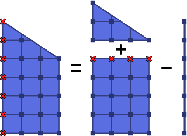
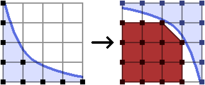
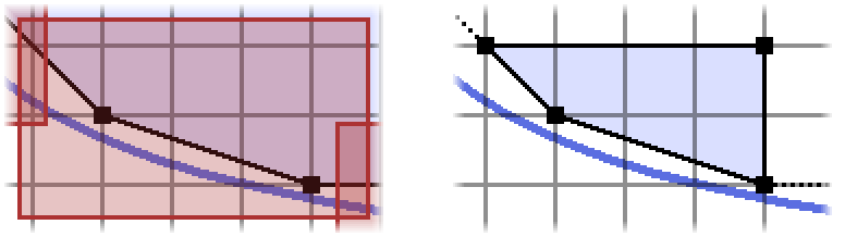
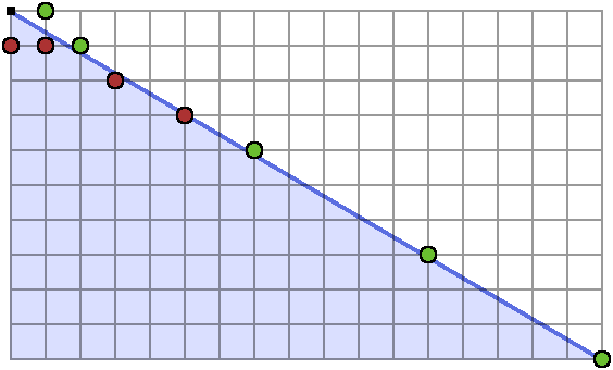
I included a diagram last time, but since this post is going to have a lot of diagrams and I want stylistic consistency, I’ve made a new one.2 Here’s what the hyperbola method is doing:
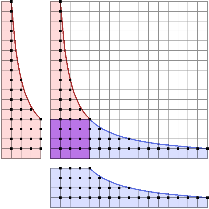
The red area on the left contains $\sum_{x \leq \sqrt{n}} \left\lfloor\frac{n}{x}\right\rfloor$ lattice points.
Because of symmetry, that’s the same number of lattice points as in the blue area on the bottom.
To get the total count, we can add those two together, so long as we subtract the number of points in the purple square, since those ones get counted twice.
This gives the answer as
\[D(n) = 2\sum_{k \leq \sqrt{n}} \left\lfloor \frac{n}{k} \right\rfloor - \lfloor\sqrt{n}\rfloor^2\]which is by itself a perfectly good algorithm to compute $D(n)$, in $O(\sqrt{n})$ time:
proc D(n: int64): int64 =
  ##Computes d(1) + ... + d(n) in O(n^(1/2)) time.
  var nsqrt = isqrt(n)
  for k in 1..nsqrt:
    result += 2*(n div k)
  result -= nsqrt*nsqrt
For small values of $n$, this simple algorithm is certainly all you need. Even at $n = 10^{17}$ it is perfectly good at only a bit over two seconds to compute the answer.
But if we want to push it to something like $n = 10^{24}$, which is more around the range we’re interested in today, we will need to do something more involved.3
Bigger Integers
Oh, right, so the thing is, we want to have our inputs and outputs much larger than $10^{19}$ which is roughly the limit of a 64-bit signed integer. If you’re doing this in something like Python where bigger integers are handled for you automatically then you don’t really have to worry about this.
The language I’ve been using so far, Nim, does not have a built in BigInt or Int128 type, which is what we’d love to be using for this. Because of that, we need to find a third party solution, or implement our own. Given that this article isn’t about how to implement fast bigger integer data types, we would opt for something third party. What I found works best is nint128, which is a package I use in my own Project Euler library. So, if you’re using Nim and want to run these functions for the large inputs they’re really built for, you can modify the code that is to follow so that it uses whatever package you choose.
Convex Hulls
The idea that I’ll be explaining in this post is something I’ve seen variously attributed to Animus in a Project Euler problem thread, who attributes the idea to Lucy_Hedgehog. If you’ve solved the relevant problem then the link will work for you and lead you to Animus’s post.
One of the better publicly available explanations of the following algorithm was written up by none other than Min_25, now living on the Internet Archive. I find that a lot of the minor details that I needed explained were basically left out of most writeups of this idea online, which made it somewhat difficult for me to realize why it actually worked. I do think the tricks that it uses are very natural, but for whatever reason it just hasn’t clicked very well in my head. So, finally, I’ve taken the time to actually attempt to explain to myself (and you) how to do it.
Returning now to thinking about counting the lattice points within a circle, our first thought should be to reduce the amount of work we have to do by using the symmetry of the circle.
Specifically, we can chop a circle up like this:
Therefore, if we count the points in the quadrant $x > 0$ and $y \geq 0$ as the quantity $L$, then the number of lattice points in the entire circle is just $4L + 1$. Let’s look at the set of integer points in this quadrant:
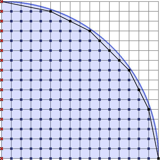
I’ve also decided to attach a black rubber band at the top left and bottom right points, and then allowed it to stretch tightly over the lattice points inside the circle. The polygon formed by the points touching this rubber band is known as the convex hull of the lattice points inside the circle. The remainder of this article is about how we can exploit these convex hulls to count the lattice points inside a shape like this.
Let’s first pretend that we have a way to obtain the points on the convex hull extremely quickly, and see how it is possible to count the number of lattice points inside the shape.
Using the Convex Hull
The simplest case, really, is when there are only one or two points on the convex hull.
It could look something like this:
As I’ve indicated, the most natural thing to do to this polygon is to break it into trapezoids4.
We obviously don’t want to be counting any lattice points twice, which would happen where the trapezoids border each other. Therefore we throw out the points on the left boundary of each trapezoid so they can slot together. Because of that, we have to count the points on the $y$-axis separately, if we wish to include them. If you look back at our circle diagrams you’ll remember we wanted to leave that axis out of the count from the start, so this is perfect.
The trapezoids that arise in this manner are defined by their upper left convex hull point $(x, y)$, and the vector $(dx, -dy)$ to the next convex hull point.5 Given these values, is it easy to count the number of lattice points in the trapezoid?
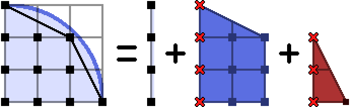
Of course! The below trapezoid has $(x, y) = (0, 6)$, and $(dx, -dy) = (3, -2)$:
We have a rectangle with $(dx+1)(y-dy)$ points, a triangle, and the left border of $y+1$ points.
We deal with the triangle in the standard way, more symmetry:
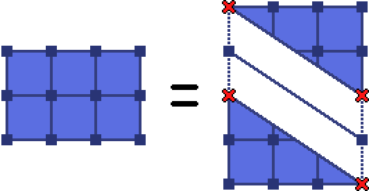
The number of lattice points in the triangle is $\frac{(dx+1)(dy+1)}{2} + 1$, since we don’t want to split those two vertices on the hypotenuse equally, we want both of them on one triangle. Notice that we’re taking advantage of $\gcd(dx, dy) = 1$, so that there are no more points on the hypotenuse of the triangle. Let’s write the trapezoid point counter now:
proc trapezoid(x0, y0, dx, dy: int64): int64 =
  ##The number of lattice points (x, y) inside the trapezoid
  ##whose points are (x0, y0), (x0+dx, y0-dy), (x0+dx, 0), (x0, 0),
  ##and such that x0 < x (so we are not counting the left border).
  result = (dx + 1) * (y0 - dy) #rectangle
  result += (((dx + 1) * (dy + 1)) shr 1) + 1 #triangle
  result -= y0 + 1 #left border
Now we are convinced that, given the points of the convex hull of a shape, we can count the lattice points inside. Here’s how a positive quarter circle looks, broken up into trapezoids:
Wait, a Hyperbola Does Not Make a Convex Set
Oops. Okay, but helpfully, we are allowed to count whatever points we want, so instead we’ll pretend we’re counting the points outside of the hyperbola. We can rotate everything around like this:
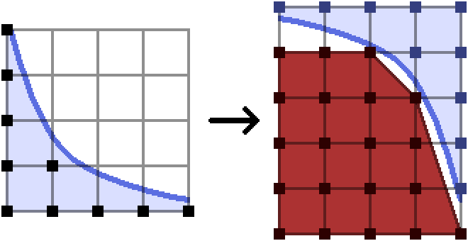
The set of points outside the hyperbola is now a nice convex set, and so we can make its convex hull and break it into trapezoids and so on, exactly as we plan to do in the case of the circle.
One important feature here which helps to make the implementation simple is the fact that I have extended the range of the function very slightly. We know the maximal $y$ value for a point we wish to count, which is at the point $(0, 4)$ in the left diagram above. When we instead consider the group of points we don’t want to count, it is most convenient to include the point $(0, 5)$.
I want you to consider instead what would happen if I didn’t extend the range of the function6:
As you can see, the convex hull of the points we don’t want to count suddenly has a range strictly smaller than that of the original set of points. It’s possible to reason about that in your code, and detect and adjust for this scenario, but who wants to do that? Not me. It was a path that led me only to despair. Meanwhile, just extending the function’s range allows us to maintain the same domain for the bad points as for the good points, so everything is nice and simple.
Once we have rotated these anti-trapezoids back so that they sit above the original shape, we can attempt to make sense of the points we actually wanted to count. Here’s how it could look:
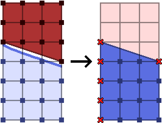
It is nearly the same situation as the regular trapezoids. They’ll be slotting together the same way as previously described, so we’ll throw out the left boundary.
This time, however, we also want to throw out the upper right corner of each generated trapezoid, since that one is actually on the boundary of the convex hull of the bad points.
We’ll come back to these anti-trapezoids later once we revisit the hyperbola case.
Finding the Convex Hull
This is the really important part of this algorithm. All of the stuff with trapezoids is completely useless if we can’t quickly find them! This section is about how we can efficiently jump from one chull (convex hull) point to the next. At this point is also when I’d like to introduce this problem more generally.
We have a function $f$ defined on some interval $[x_0, x_1]$ which takes non-negative real values.
Additionally, we assume that $f$ has nonpositive derivative and second derivative on the interior of the interval, so that the set of points $(x, y)$ with $x_0 \leq x \leq x_1$ and $0 \leq y \leq f(x)$ forms a convex set.
In the circle case, we had $f(x) = \sqrt{n - x^2}$ on the interval $[0, \sqrt{n}]$.
From this point on when I make mention to ‘the shape’ or ‘the blob’, I’m referring to the convex set with boundaries described above. Hopefully that’s easy enough to follow.
Anyway, we want to be able to handle this counting problem for whatever $f$ we have, so I’ll phrase it in general when I can. The diagrams from here on will mostly be the circle case, since that one is nicer.
Let’s suppose we are at a convex hull point $(x, y)$ and want to find the next.
Generally there will be lots of options for vectors $(dx, -dy)$ to choose to get to the next point. In the above, we should clearly prefer the vector $(5, -3)$ over the vector $(3, -2)$ since the former is shallower7. The next point on the convex hull will be at $(x+dx, y-dy)$ where $(dx, -dy)$ is the shallowest vector such that the resulting point fits in the blob we are considering. So the question becomes, how can we quickly find this shallowest $(dx, -dy)$?
Stern-Brocot Binary Search Tree
Skip this section if you think the use of SB tree is obvious. This was one of the parts which was most non-obvious to me, so I assume there will be some other people who also think it’s not obvious.
Consider maintaining intervals such that we know the next slope $dy/dx$ is somewhere in the range $[a, b]$.
We can start with $[\frac{0}{1}, \frac{1}{0}]$, the interval of all positive reals including infinity. The slope $\frac{1}{0}$ here represents moving one unit directly downwards, of course, and we don’t really intend to divide by zero.
We want to refine our search over the interval $[\frac{a}{b}, \frac{c}{d}]$ by splitting it into two parts.
Pretend that we don’t know exactly how we’re going to do that yet, so the midpoint is just some mysterious reduced fraction $\frac{e}{f}$ in the interval.
The most important thing we have to be able to do is determine if the shallowest $dy/dx$ such that $(x+dx, y-dy)$ fits inside our shape can be found in a given interval.
We will use the following nice idea:
Requirement 1. Let an interval of reduced fractions $[\frac{a}{b}, \frac{c}{d}]$ be given, and suppose $p/q$ is any reduced fraction in the interior of this interval.
If $(x+q, y-p)$ fits in the blob, then $(x+d, y-c)$ also will fit.
This seems rather strange, since $c/d$ is steeper than $p/q$ we may expect $c/d$ could be too large to fit. But it turns out that we can find a system of intervals such that this requirement holds, and moreover there’s only one way to do it.
For now, we’ll motivate this requirement by showing how we use it.
Since we are looking for the shallowest possible slope, suppose we have narrowed our search down to the first interval of the finite sequence
\[[\frac{a_1}{b_1}, \frac{a_2}{b_2}] \cup [\frac{a_2}{b_2}, \frac{a_3}{b_3}] \cup \ldots = [\frac{a_1}{b_1}, \frac{1}{0}]\]where we have previously broken down $[\frac{0}{1}, \frac{1}{0}]$ into some number of parts and perhaps thrown away some parts we now know to be too shallow to include.
First, just see if we can use $\frac{a_1}{b_1}$ as a slope, since it’s obviously shallowest.
If $(x+b_1, y-a_1)$ fits in the blob, then jump to that point, and repeat until $(x+b_1, y-a_1)$ no longer fits. The shallowest slope we can use after this point is now strictly steeper than $\frac{a_1}{b_1}$, so we need to decide what to do with the interval $[\frac{a_1}{b_1}, \frac{a_2}{b_2}]$.
We should now test the steeper endpoint, and see whether $(x+b_2, y-a_2)$ is in the blob.
If it isn’t, then we throw out the entire interval, since the Requirement for the intervals under consideration implies that no reduced fractions on the interior will fit either.
If, however, $(x+b_2, y-a_2)$ does fit, then there may be some shallower slope in the interior of the interval $[\frac{a_1}{b_1}, \frac{a_2}{b_2}]$ that we should prefer, so we have to split the interval in two and then examine the shallower part. We should hope to someday encounter the shallowest possible slope as an endpoint, so we should also require
Requirement 2. Every reduced fraction should eventually be found as an endpoint of the intervals in our system.
There is a very small problem, which is that we don’t know when to stop splitting an interval, in the case that $\frac{a_2}{b_2}$ is actually the shallowest possible slope that we can use. The intervals can always be split, and so we would just split with reckless abandon forever.
We will deal with this shortly once we figure out what the intervals should be.
Lemma 1. For Requirement 1 to hold for an interval $[\frac{a}{b}, \frac{c}{d}]$, it must be true that any reduced fraction $p/q$ in the interior of the interval must have $p>c$ and $q>d$.
Proof. Since our interval choices should work no matter what the blob looks like, we can choose a specific one which helps us prove the lemma. The most helpful one to choose is the set of points $(x, y)$ with $0 \leq x \leq q$ and $0 \leq y \leq p - \frac{p}{q}x$, which forms a triangle like this:
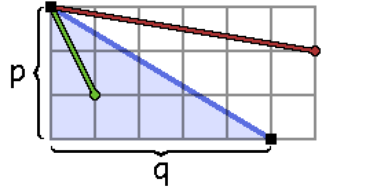
Here I’ve chosen the parameters $\frac{p}{q} = \frac{3}{5}$, and I’ve also added the endpoints of the interval $[\frac{1}{6}, \frac{2}{1}]$.
Requirement 1 says that the steeper endpoint (here $\frac{c}{d} = \frac{2}{1}$) should be such that $(0+d, p-c)$ is inside the triangle, since $(q, p)$ is in the blob. Actually this makes things very obvious, since any point $\frac{c}{d}$ we could use as an endpoint will necessarily land inside the triangle, and so we have $c \leq p$ and $d \leq q$.
Now let’s see how we can use this to determine our system of intervals.
Lemma 2. Let $[\frac{a}{b}, \frac{c}{d}]$ be an interval, and $\frac{p}{q}$ the fraction in the interior with the smallest denominator, and then if there are multiple options, the one with the smallest numerator. Then the interval should be split at or before $\frac{p}{q}$.
Proof. By requirement 1, we have $p \geq c$ and $q \geq d$.
If $p/q$ ends up in the shallower of the two intervals we split into, then there will be a problem.
The steeper endpoint would have a denominator or numerator larger than that of $p/q$, violating Requirement 1. Therefore, we have to split the interval either at $p/q$ or at some more complicated fraction coming before $p/q$. $\newcommand{\proofqed}{\quad\quad\square}\proofqed$
Alright, enough beating around the bush.
The Stern-Brocot tree splits the interval $[\frac{a}{b}, \frac{c}{d}]$ at the slope $p/q$ described above. Moreover, starting from $[\frac{0}{1}, \frac{1}{0}]$, we get intervals $[\frac{a}{b}, \frac{c}{d}]$ who split at $\frac{p}{q} = \frac{a+c}{b+d}$, the mediant of the two endpoints. These will always be reduced fractions. The sizes of the numerators and denominators imply that these choices will give us intervals satisfying Requirement 1. Also, every reduced fraction will show up as an endpoint of an interval, which is Requirement 2. It all works out very well, and people who were previously familiar with Stern-Brocot would say this is the most natural way to arrange reduced slopes into a binary search structure8. This is the correct way to search for the next slope.
If you want to learn more about the Stern-Brocot tree, and its relation to continued fractions and best rational approximations, I recommend you read this from algmyr, adamant, and others on cp-algorithms, and this other interesting article written by adamant.
It is widely applicable and a good thing to know about.
There was one thing we briefly considered a few moments ago which we now have to deal with.
We were considering the shallowest interval $[\frac{a}{b}, \frac{c}{d}]$, and had assumed we had jumped by $(b, -a)$ as much as possible, such that $(x+b, y-a)$ no longer fits in the blob. We need a way to determine when we cannot gainfully split this interval up any further to search for shallower slopes than $\frac{c}{d}$.
Now, though, we are aware that the point we split the interval at is $\frac{a+c}{b+d}$.
If this slope fails, we would have to split $[\frac{a+c}{b+d}, \frac{c}{d}]$ at $\frac{a+2c}{b+2d}$, and so on.
The slopes we consider are all of the form $(b+kd, a+kc)$ for integer $k \geq 1$, and we need a way to determine when none of these will work.
One simple idea is to simply stop once $a+c$ or $b+d$ exceed known bounds on the size of the shape, like its height or width, but it turns out that we would consider an unhealthy number of slopes this way.
A more complicated idea, but one which is able to cut out much sooner, is to consider the slope of the boundary of the blob near the point $(x+b+d, y-a-c)$. First we check that point to make sure it’s not in the blob. Then, if the boundary of the blob is receding faster than we can approach it by taking mediants towards $\frac{c}{d}$, we will have no hope of ever meeting the blob again.
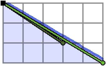
I’ve pictured an example of this behavior.
Above, we are considering splitting the interval $[\frac{1}{3}, \frac{1}{2}]$.
The first mediant $\frac{2}{5}$ is pictured as the extended red ray, which does not land in the blob. Even worse, successive mediants $\frac{3}{7}, \frac{4}{9}$, etc, which would be the endpoints of further splits towards $\frac{1}{2}$, lie along the higher of the two dark blue rays I drew. The bottom ray is heading downwards faster than that, though, and so there’s no way any shallower slope than $\frac{1}{2}$ will work.
When we get to this point in the slope search, we can throw out this interval, since $\frac{1}{2}$ will be the shallower endpoint of the next interval on our list. This cutoff behavior is summarized as
Slope Search Pruning. Suppose $[\frac{a}{b}, \frac{c}{d}]$ is a slope search interval.
Also assume $\frac{a}{b}$ has been used as much as possible, so $(x+b, y-a)$ no longer fits.
If $x+b+d > x_1$ is out of bounds, or if $y-a-c < 0$ is out of bounds, abandon the interval, since the numerators and denominators of the mediants will only increase.
If $f’(x+b+d) \leq -\frac{c}{d}$, the blob is receding faster than we are able to catch up to it.
We can determine that no further mediants work, and we can abandon the interval.
Otherwise, we may possibly find a shallower slope than $\frac{a}{b}$ somewhere.
In this case, split the interval at $\frac{a+c}{b+d}$.
Generic Implementation
It’s time…
The algorithm accepts an initial point (x0, y0) on the convex hull and a final coordinate x1. It’s a little nicer to give it x1 instead of leaving its value implied by the restrictions of the next functions, since this way we can cut the sum a little earlier without modifying the rest of the inputs.
We specifically require the use of inside(x, y) which is able to quickly determine whether a given point $(x, y)$ is inside the blob, and another function called prune(x, y, dx, dy) which determines whether any point $(x+n\cdot dx, y - n\cdot dy)$ could potentially land in the blob.
That should be all we need.
The function will return the edges of the upper boundary of the convex hull as (x, y, dx, dy), which also determines the trapezoids with points (x, y), (x+dx, y-dy), (x+dx, 0), (x, 0).
Here’s how it looks in Nim.
iterator chullConcave(x0, y0: int64,
              x1: int64,
              inside: (proc (x, y: int64): bool),
              prune: (proc (x, y, dx, dy: int64): bool)): (int64, int64, int64, int64) =
  ##Finds the convex hull of integer points
  ##with xInit <= x <= x1, and 0 <= y <= f(x), where f is concave.
  ##Yields (x, y, dx, dy),
  ##where the next edge is from (x, y) to (x+dx, y-dy).
  ##(x0, y0) is the top left point of the hull.
  ##A point is in the shape iff inside(x, y).
  ##Also provide prune(x, y, dx, dy) which returns whether f'(x) <= -dy/dx.
  ##This works for f'(x) <= 0 and f''(x) <= 0.
  #---
  var (x, y) = (x0, y0)
  var stack = @[(0'i64, 1'i64), (1'i64, 0'i64)]
  #stack of slopes (dx, dy) = -dy/dx
  #always kept in order of steepest slope to shallowest slope
  #adjacent values form slope search intervals
  while true:
    var (dx1, dy1) = stack.pop()
    #(dx1, dy1) is the shallowest possible slope in the convex hull
    if dx1 == 0: #going straight down
      #no need to make any silly looking chull points
      break
    #use the slope -dy1/dx1 as much as possible
    while x + dx1 <= x1 and inside(x + dx1, y - dy1):
      yield (x, y, dx1, dy1)
      x += dx1
      y -= dy1
    #test if we are at the end already..
    if y == 0: break

    #get current slope search interval
    var (dx2, dy2) = (dx1, dy1)
    while stack.len != 0:
      (dx1, dy1) = stack[^1]
      #here, [dy2/dx2, dy1/dx1] forms the shallowest slope search interval
      if x + dx1 <= x1 and inside(x + dx1, y - dy1):
        break #by requirement 1, this interval contains the next slope
      #otherwise it is useless, so we discard the interval,
      #while maintaining the steeper endpoint
      discard stack.pop
      (dx2, dy2) = (dx1, dy1)
    if stack.len == 0: break #probably unecessary to add this here

    #the shallowest slope is somewhere in [dy2/dx2,dy1/dx1]
    while true:
      var (mx, my) = (dx1 + dx2, dy1 + dy2) #interval mediant
      if x + mx <= x1 and inside(x + mx, y - my):
        (dx1, dy1) = (mx, my)
        stack.add (mx, my)
        #stack has the intervals [my/mx, dy1/dx1], [dy1/dx1, ..], ...
        #active interval is [dy2/dx2, my/mx]
      else:
        if x + mx > x1 or prune(x + mx, y - my, dx1, dy1):
          #slope search prune condition
          #the intervals [(dy2+n*dy1)/(dx2+n*dx1), dy1/dx1] never work
          #fully discard dy2/dx2 and therefore the interval [dy2/dx2,dy1/dx1]
          break
        #refine the search to [my/mx, dy1/dx1]
        (dx2, dy2) = (mx, my)
    #the search is over
    #top of the stack contains the next active search interval
The actual code is very short, I have just labelled all of the ideas to try to make it as easy to reference as possible. We’ll talk about the runtime of this function later, but for now let’s use it:
proc concaveLatticeCount(x0, y0: int64,
              x1: int64,
              inside: (proc (x, y: int64): bool),
              prune: (proc (x, y, dx, dy: int64): bool)): int64 =
  ##Uses the chull edges to find the number of lattice points
  ##under a decreasing concave function.
  ##This is for f' <= 0 and f'' <= 0.
  ##Does NOT include points at the border with x = xInit.
  ##The point (x0, y0) is the top left point satisfying y0 <= f(x0).
  for (x, y, dx, dy) in chullConcave(x0, y0, x1, inside, prune):
    result += trapezoid(x, y, dx, dy)
I’ve called it concaveLatticeCount because the boundary function is concave.
Here, we give the same information as before, but now we’re adding up the number of lattice points inside of each generated trapezoid. As discussed before, this does not include the count of points on the left $x$-boundary, with x = xInit, so if you wanted to include those, please do not forget them.
Counting a Circle’s Lattice Points
Let’s apply the function we made to the problem of counting all the lattice points inside a circle.
This is the sum $R(n) = \sum_{0 \leq k \leq n} r_2(k)$, if you forgot.
Recall from earlier that we will count the number $L$ of lattice points in the circle such that $x > 0$ and $y \geq 0$, and then get the answer as $4L+1$.
The function inside(x, y) is easy, we can just check $x^2 + y^2 \leq n$.
When it comes to interval pruning, we are given a point $(x, y)$ with integer coordinates which failed to land inside the shape, and we have a slope $-dy/dx$, and we need to test $f’(x) \leq -dy/dx$.
Implicit differentiation of the curve $x^2 + f(x)^2 = n$ gives $f’(x) = -x/f(x)$.
Certainly if $-x/y \leq -dy/dx$, then also $-x/f(x) \leq -dy/dx$ since $y > f(x)$.
So we can actually just check $dx \cdot x \geq dy \cdot y$ which is easier than doing floating points or dealing with unnecessarily ugly numbers. It’s possible we could cut out earlier but this is fine.
Here’s an implementation:
proc circleLatticePointCount(n: int64): int64 =
  let sqrtn = isqrt(n)
  proc inside(x, y: int64): bool =
    return x*x + y*y <= n and y >= 0
  proc prune(x, y, dx, dy: int64): bool =
    if x > sqrtn or y <= 0: return true
    return dx * x >= dy * y
  var L = concaveLatticeCount(0, sqrtn, sqrtn, inside, prune)
  return 4*L + 1
It takes about 0.03 seconds for $n = 10^{18}$, compared to the 1 second the easy algorithm gives.
Written using a library with Int128, it uses about a half a second for the same limit due to the overhead.
Once we are able to plug in larger $n$, though, this algorithm does much better.
It takes about 38 sec to compute the number of points $x^2 + y^2 \leq 10^{24}$.
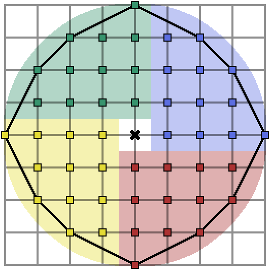
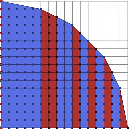
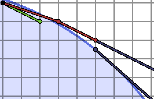
Here is a visualization of the algorithm is actually doing.
The green rays are slopes on the stack which form endpoints of search intervals, and the red rays are those which fail to fit in the blob. Once a convex hull point is determined I’ve added it as a black vertex.
As a short final aside for the circle case, it is possible to get a small but significant runtime improvement by restricting the segment of the quarter circle slightly to make better use of symmetry.
We can sum over $0 < x \leq \sqrt{n/2}$ and use the symmetry of the circle over the line $y = x$ to compute the answer as follows:
proc circleLatticePointCount2(n: int64): int64 =
  let sqrtn = isqrt(n)
  proc inside(x, y: int64): bool =
    return x*x + y*y <= n and y >= 0
  proc prune(x, y, dx, dy: int64): bool =
    if x > sqrtn or y <= 0: return true
    return dx * x >= dy * y
  var x1 = isqrt(n div 2)
  var L = 1 + sqrtn + concaveLatticeCount(0, sqrtn, x1, inside, prune)
  L = (2*L - (1+x1)*(1+x1)) - sqrtn - 1
  return 4*L + 1
There is one more optimization we make later which I can also apply to this case, to reduce the memory used by the stack. I’ll get into that after we talk about the hyperbola case. Anyway, with this extra optimization, switching to Int128 and parallelizing, this computes $R(10^{24})$ in 2.6 seconds, compared to 8.4 seconds to sum over all $0 < x \leq \sqrt{n}$. To compute $R(10^{36})$ this way would take about 7-8 hours on my cpu.
Counting a Hyperbola’s Lattice Points
Now we’re going to actually deal with the anti-trapezoids from earlier.
We have a function $f$ defined on some interval $[x_0, x_1]$ which takes non-negative real values.
This time, the function we’re curious about is $f(x) = n/x$, which is not concave.
A convex function like this, for which the set of points underneath it does not form a convex set9, has a nonpositive derivative but a nonnegative second derivative on the interior of the interval. The set of points above this kind of function does make a convex set, so we’ll be hopping around the set of points $(x, y)$ with $y > f(x)$.
I indicated earlier that we can visualize this by rotating the function around, and applying the convex hull hopping algorithm there, then rotating back. To avoid unnecessary arithmetic (a bunch of subtractions), we can just write a slightly modified version of the previous chullConcave algorithm.
We’ll be starting at the point $(x_0, y_0 + 1)$ which is the first point above the boundary curve $f$.
At each stage, rather than looking for the shallowest slope which fits inside the blob, we’ll find the steepest slope which does not fit inside the blob. This will traverse the same set of points that the rotated function would’ve generated, had we simply plugged it into chullConcave from before.
All of the analysis is the same as what we’ve already done once before.
The condition for pruning an interval is also helpfully extremely similar.
Rather than checking $f’(x) \leq -dy/dx$, we should check $f’(x) \geq -dy/dx$.
Here’s the code:
Nim Code
iterator chullConvex(x0, y0: int64,
              x1: int64,
              inside: (proc (x, y: int64): bool),
              prune: (proc (x, y, dx, dy: int64): bool)): (int64, int64, int64, int64) =
  ##Finds the convex hull of integer points
  ##with xInit <= x <= x1, and f(x) < y, where f is convex.
  ##Yields (x, y, dx, dy),
  ##where the next edge is from (x, y) to (x+dx, y-dy).
  ##(x0, y0) is the top left point of the hull, and satisfies f(x0) < y0.
  ##A point is in the shape iff inside(x, y).
  ##Also provide prune(x, y, dx, dy) which returns whether f'(x) >= -dy/dx.
  ##Note the order of the above inequality compared to chullConcave.
  ##This works for f'(x) <= 0 and f''(x) >= 0.
  #---
  var (x, y) = (x0, y0)
  var stack = @[(1'i64, 0'i64), (0'i64, 1'i64)]
  #stack of slopes (dx, dy) = -dy/dx
  #always kept in order of shallowest slope to steepest slope
  #adjacent values form slope search intervals
  while true:
    var (dx1, dy1) = stack.pop()
    #(dx1, dy1) is the steepest possible slope in the convex hull
    #dx1 == 0 should never happen in the case we deal with
    #use the slope -dy1/dx1 as much as possible
    while x + dx1 <= x1 and not inside(x + dx1, y - dy1):
      yield (x, y, dx1, dy1)
      x += dx1
      y -= dy1
    #test if we are at the end already..
    #again this is not going to happen for the case we deal with
    if y == 0: break

    #get current slope search interval
    var (dx2, dy2) = (dx1, dy1)
    while stack.len != 0:
      (dx1, dy1) = stack[^1]
      #here, [dy2/dx2, dy1/dx1] forms the steepest slope search interval
      if x + dx1 <= x1 and not inside(x + dx1, y - dy1):
        break #by requirement 1, this interval contains the next slope
      #otherwise it is useless, so we discard the interval,
      #while maintaining the shallower endpoint
      discard stack.pop
      (dx2, dy2) = (dx1, dy1)
    if stack.len == 0: break #probably unecessary to add this here

    #the steepest slope is somewhere in [dy2/dx2,dy1/dx1]
    while true:
      var (mx, my) = (dx1 + dx2, dy1 + dy2) #interval mediant
      if x + mx <= x1 and not inside(x + mx, y - my):
        (dx1, dy1) = (mx, my)
        stack.add (mx, my)
        #stack has the intervals [my/mx, dy1/dx1], [dy1/dx1, ..], ...
        #active interval is [dy2/dx2, my/mx]
      else:
        if x + mx > x1 or prune(x + mx, y - my, dx1, dy1):
          #slope search prune condition
          #the intervals [(dy2+n*dy1)/(dx2+n*dx1), dy1/dx1] never work
          #fully discard dy2/dx2 and therefore the interval [dy2/dx2,dy1/dx1]
          break
        #refine the search to [my/mx, dy1/dx1]
        (dx2, dy2) = (mx, my)
    #the search is over
    #top of the stack contains the next active search interval
And, as before, we have
proc convexLatticeCount(x0, y0: int64,
              x1: int64,
              inside: (proc (x, y: int64): bool),
              prune: (proc (x, y, dx, dy: int64): bool)): int64 =
  ##Uses the chull edges to find the number of lattice points
  ##under a decreasing convex function.
  ##This is for f' <= 0 and f'' >= 0.
  ##Does NOT include points at the border with x = xInit.
  ##The point (x0, y0) is the top left point satisfying f(x0) < y0.
  for (x, y, dx, dy) in chullConvex(x0, y0, x1, inside, prune):
    result += trapezoid(x, y, dx, dy) - 1
At last we can implement the code which computes $D(n)$.
To decide about prune, we differentiate $xf(x) = n$ to obtain $xf’(x) + f(x) = 0$, and so $f’(x) = -f(x)/x$. The function prune accepts a point $(x, y)$ with $y \leq f(x)$ which fails to be strictly above the boundary curve, and we must check if $f’(x) \geq -dy/dx$ for the slope $(dx, dy)$.
This works out to verifying $f(x)dx \leq xdy$. We can get away with checking $ydx \leq xdy$.
Here it is put together:
proc hyperbolaLatticePointCountBad(n: int64): int64 =
  let nrt = isqrt(n)
  var x0 = 1'i64
  var y0 = n div x0
  var x1 = nrt
  proc inside(x, y: int64): bool =
    return x*y <= n
  proc prune(x, y, dx, dy: int64): bool =
    return dx * y <= dy * x
  var L = convexLatticeCount(x0, y0 + 1, x1, inside, prune)
  L += 1 + y0 #add in the points on the left boundary
  L -= x1 #get rid of the points on the x-axis
  return 2*L - nrt*nrt
If you test this for $D(10^{17})$, unfortunately, you will have to wait for a while. It’s a shame, but actually, the way the chull algorithm is written gives us a terrible $\Theta(n)$ runtime for this case. That’s significantly worse than the easy method from earlier, which ran in $O(\sqrt{n})$ time. So what’s happening here?
What’s Happening Here
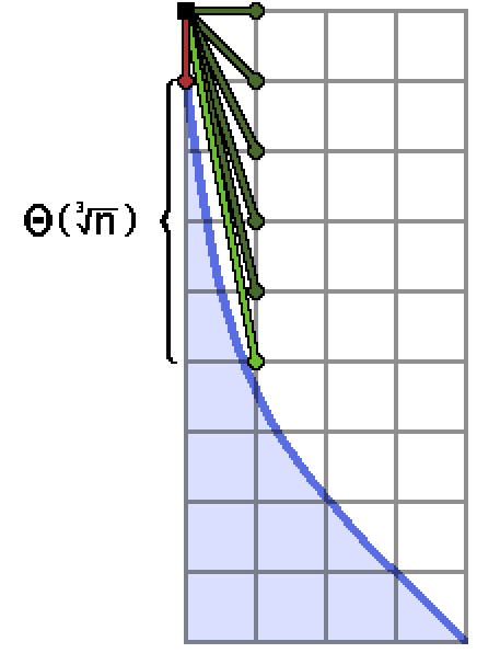
It is helpful to examine the first few steps of the convex hull walk on a shape which has a large section which is extremely shallow or steep, like the ends of the hyperbola:
I’ve labeled a very wide, flat section of this boundary, which has length $\Theta(n)$ (maybe like $n/2$).
This step, which takes forever to run, is descending the Stern-Brocot tree.
We’re calculating mediants of the interval $[\frac{0}{1}, \frac{1}{0}]$ towards the shallower end, and every single time, that mediant fits. So we keep splitting the interval, descending to $[\frac{0}{1}, \frac{1}{1}]$, then $[\frac{0}{1}, \frac{1}{2}]$, then $[\frac{0}{1}, \frac{1}{3}]$, and so on. Our interval shrinks, in this case, until we get to about $[\frac{0}{1}, \frac{1}{\lfloor n/2 \rfloor}]$, at which point we have $\Theta(n)$ endpoints sitting in the stack, which is completely horrible.
The same thing would necessarily happen at an extremely steep section of a curve.
So, if we’re aiming to count the number of points under a certain curve, it is beneficial to completely cut out the sections where the slope is extremely high. Helpfully, when this happens, the function’s value will be changing very quickly, so these regions should be relatively small. The regions where the slope is changing extremely slowly can be handled by summing over $y$ rather than $x$, if necessary.
More relevant information is mentioned as a footnote in Min_25’s writeup:
$\sigma_0(n)$ の総和に対応します。$f^{\prime\prime}(x) = 2n/x^3$ なので、
$\sqrt[3]{2n} < x \leq \sqrt{n}$ の部分について、凸包を取ります。
They calculate the second derivative of $f$, and then deduce that you are supposed to use the convex hull strategy on the domain $\sqrt[3]{2n} < x \leq \sqrt{n}$. They elaborate a bit earlier in their article:
ただ、これらの関数 ($f(x)= \sqrt{n^2 - x^2}$, $f(x)=n/x$) は傾きが緩やかに変化する $x$ の範囲(例えば、$\lvert f^{\prime\prime}(x)\rvert<1$ の範囲)が比較的広く、整数点集合 $P(n):={(x,\lfloor f(x)\rfloor) \mid 1 \leq x \leq n}$ に対する凸包の端点数は少ないです。
Roughly, the regions where the slope is changing slowly, for instance with $\lvert f^{\prime\prime} \rvert < 1$, are relatively wide. As a result, the number of vertices on the convex hull on those regions is comparatively low.
Ideally this is the case, since then we can hop large distances without generating many trapezoids.
On the other hand, if the slope of the boundary is too steep or too shallow, we get a situation like pictured above, in which we need to calculate too many mediants to proceed with the chull walk.
For the hyperbola, we’ll avoid the initial region of extremely high slope by computing the sum $\sum \left\lfloor \frac{n}{x}\right\rfloor$ over $1 \leq x \leq (2n)^{1/3}$ separately, and then give the rest of the region up to $\sqrt{x}$ to the hull hopper.
Here’s how it looks:
proc hyperbolaLatticePointCount(n: int64): int64 =
  let nrt = isqrt(n)
  var x0 = iroot(2*n, 3)
  var y0 = n div x0
  var x1 = nrt
  proc inside(x, y: int64): bool =
    return x*y <= n
  proc prune(x, y, dx, dy: int64): bool =
    return dx * y <= dy * x
  var L = convexLatticeCount(x0, y0 + 1, x1, inside, prune)
  for i in 1..x0: #add in the points with x <= x0
    L += (n div i) + 1
  L -= x1 #get rid of the points on the x-axis
  return 2*L - nrt*nrt
Now it finishes for $n = 10^{17}$ in about 0.06 seconds, compared to over two seconds for the simple algorithm. It overflows for $10^{18}$ (oops) but when converted to Int128s, it finishes calculating $D(10^{24})$ in about 3 minutes. The standard method would take hours without some other strange optimizations.
At last, we’ve made our $R(n)$ and $D(n)$ faster!
But there’s a question burning in our minds, which is
How Many Trapezoids?
Not that many.
One simple result in the desired direction is a comment by dacin21 on this Codeforces blog post:
Lemma 3. A convex lattice polygon with coordinates in $[0, N]$ has at most $O(N^{2/3})$ vertices.
It turns out, after researching this topic for a while, this sort of idea has been a popular one to study.
A more flexible theorem was proved by Arnol’d in a paper titled Statistics of Integral Convex Polygons:
Lemma 4. The number of vertices of a convex polygon of area $\mu/2$ with vertices at integral points of the plane does not exceed $16\mu^{1/3}$.
It’s phrased in terms of $\mu$, twice the area of the polygon, since that is necessarily an integer (see Pick’s Theorem). The previous theorem on the number of vertices of a convex lattice polygon follows by noticing that the area of a convex polygon living in $[0, N]^2$ is certainly at most $N^2$, so it must have at most $16*2^{1/3} N^{2/3}$ vertices.
Another paper, by Stanley Rabinowitz, improves the constant term considerably. I highly recommend reading it, as the result is intriguing and the proof is short and beautiful. The obtained result is
Lemma 5. If $A$ is the area of a convex lattice $n$-gon, then
\[A > \frac{n^3}{8\pi^2}\]
The inequality by Arnol’d can be phrased as $A > n^3 / 8192$, for comparison.
When we attempt to apply a result of this type to bound the number of trapezoids generated by our chull algorithms, we have a very small problem. The convex polygons in these theorems do not allow any straight angles. That is, it is not allowed for three consecutive vertices of the polygon to be collinear. If it were allowed, we could form a big right triangle with slope $-1$ which would have area approximately $n^2/2$ and about $n$ vertices.
Clearly, the shapes we’re working with are curvy enough that their boundaries should not have that many repeated slopes (which generate these collinear vertices), but we would like to prove it.
For now, we can easily apply the mentioned theorems to show that the number of distinct slopes is small in the circle case, by just estimating its area. A quarter circle of radius $r$ has area $\pi r^2 / 4$, so
The number of slopes on the convex hull of the lattice points inside a circle of radius $r$ is fewer than $2^{1/3} \pi r^{2/3}$. Thus, to calculate $R(n)$ we need fewer than $2^{1/3} \pi n^{1/3}$ slopes.
Applying these results to the hyperbola is slightly more involved.
The convex shape involved for $xy = n$ has an area not greater than $n^2$, which gives us a bound of $O(n^{2/3})$ on the number of slopes required, which is pretty horrible.
We can do slightly better by using the bounding rectangle $[(2n)^{1/3}, \sqrt{n}] \times [\sqrt{n}, 2^{-1/3} n^{2/3}]$ which covers the short segment of the hyperbola that we actually feed to the chull algorithm.
It has an area of $O(n^{7/6})$, which then tells us that the number of distinct slopes used in the convex hull over that interval is $O(n^{7/18})$.
The best known (?) estimate is not actually very hard to obtain from here.
First, Min_25 presents the bound $O(n^{1/3} \log(n))$ on the number of trapezoids. They do include a small question mark since they do not provide a proof or a link to a proof. The correct idea is not too difficult to find, and the logarithmic factor makes a very good hint if you want to try it yourself.
One proof of the $O(n^{1/3} \log(n))$ vertex count appears in a paper by David Alcántara and others, titled On the convex hull of integer points above the hyperbola. Their paper works on a more general hyperbola, and follows many of the same ideas I’ve presented in this post so far. They even include a description of an algorithm to produce the same points we’ve been interested in producing, so their paper is a good read if you want some more convex hull content.
I will briefly paraphrase the key ideas here.
Remember that we obtained a much improved vertex bound by reducing to a smaller segment of the hyperbola, which was covered by a rectangle with smaller area, which led to a smaller vertex count by Lemma 4-5. We can use nicely chosen rectangles in a similar way to obtain what seems to be optimal.
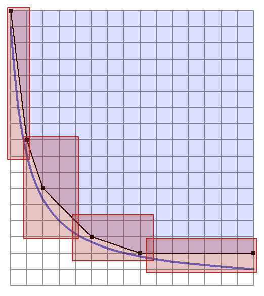
Above is a very approximate representation of what we aim to accomplish.
We can look inside each rectangle specifically and see how the points inside behave.
Shown is one rectangle (we will describe how they are chosen shortly) and the portion of the convex hull which lies inside, on the left. Considering all of the lattice points which lie inside the rectangle and strictly above the hyperbola, we can also take their convex hull, which is shown on the right10.
It seems we have more points.
Lemma 6. A vertex $v$ of the convex hull above the hyperbola is also a vertex of the convex hull of the restricted set of points inside a rectangle containing $v$.
Basically, looking at the different segments of the hyperbola will not mysteriously forget to use one of the chull points by improving the shape of the polygon in some way. We can only make the polygons more pointy by chopping them up like this. The proof of this is very straightforward:
Proof. Given a set of points $A \subset \mathbb Z^2$ and a subset $B \subset A$, the convex hull of $B$ is a subset of the convex hull of $A$. If a vertex $v$ were an interior point of the convex hull inside a rectangle, then it would also be an interior point of the entire convex hull above the hyperbola. Similarly if $v$ were a boundary point of the convex hull inside a rectangle, then it would necessarily be a boundary point or interior point of the larger convex hull. $\proofqed$
This justifies counting the number of vertices of the convex hull of the points inside each rectangle and above the hyperbola. The total of these would constitute a (perhaps loose) limit on the number of vertices of the convex hull we’re interested in. Also notice that the same strategy of proof, and a similar bound, would apply to whatever hyperbola segment we really care about here.
Now, following Alcántara, we choose the $x$ coordinates of the rectangles as a geometric series. The specifics sort of don’t really matter for us, as we’re not looking for a super specific estimate. Actually, let’s look at the expression that Alcántara produces, just for fun:
… Hence, the total number of vertices (including the first and last) is at most
\[\left(\frac{2^8\pi^2(k-1)^2}{k}m\right)^{\frac{1}{3}} (\log_k m + 2)\]
Here, $k \geq 2$ is the geometric series ratio that determines the rectangle coordinates, which has some other restrictions, and $m$ is related to our $n$ by the determinant of the chosen lattice. In our case the lattice is just $\mathbb Z^2$ so $m = n$ and we get something $O(n^{1/3} \log(n))$ but wow, complicated looking.
Anyway, we choose whatever geometric series looking thing we want, say $2^0, 2^1, \ldots, 2^{\ell - 1}, 2^\ell$.
We choose $\ell$ such that $2^{\ell - 1} < n \leq 2^\ell$, so we have $\ell = O(\log n)$.
Now we form a sequence of points $r_0, r_1, \ldots, r_\ell$ as $r_i = (2^i, n/2^i)$, which are all on the hyperbola. Note that these are likely not lattice points, and they may extend well past the end of the hyperbola, but who cares.
We will form $\ell$ rectangles from these points. In our case, we took the convex hull of the lattice points strictly above the hyperbola, whereas Alcántara also included the points on the hyperbola. There’s not much difference, but that means for me it’s a bit simpler to have slightly taller rectangles.
Rectangle $i$, for $0 \leq i < \ell$, will have its top left point at $r_i + (0, 1)$, and its bottom right point at $r_{i+1}$.
This way, every point $(x, y)$ which is at most one unit above the hyperbola will be covered by a rectangle. This is enough to ensure we’ve covered the entire convex hull we are thinking about.
Rectangle $i$ has an area of
\[\begin{align*} (2^{i+1} - 2^i) * \left(\frac{n}{2^i} + 1 - \frac{n}{2^{i+1}}\right) &= 2^i * \left(\frac{n}{2^{i+1}} + 1\right)\\ &= \frac{n}{2} + 2^i \leq \frac{3}{2}n \end{align*}\]Plenty good enough, as now the convex hulls inside of each rectangle have $O(n^{1/3})$ vertices each, for a total of $O(n^{1/3} \log(n))$ vertices for the hyperbola, as desired.
If you want a more detailed analysis of this idea, please read the paper by Alcántara and others.
My work here was somewhat sloppy, but this article is long enough as it is, and we somehow have more I want to get to.
So, we’ve figured out the order of magnitude of the number of slopes on the convex hull for the circle and for the hyperbola. Obviously in the general case you’d have to do your analysis tailored to the function you’re using. But even now, after all this work, there’s a question burning in our minds, which is
Really, How Many Trapezoids?
It seems more difficult to obtain an estimate for the number of trapezoids, since each of the $O(n^{1/3} \log(n))$ different slopes may be used multiple times. We can do an experiment though, since we can just pick a very large $n$ and make some observations about the convex hull.
The statistics we’ll measure are the number of distinct slopes used, the number of trapezoids, the maximum multiplicity of a single slope, and maximum length of the stack of slope search interval endpoints during the algorithm. After that we’ll look at the counts of each slope multiplicity.
Remember that this data is for the section of the hyperbola with $\sqrt[3]{2n} \leq x \leq \sqrt{n}$.
Let’s start with a few modest $n$, and see how things look.
| n | Slopes | Trapezoids | Avg Multiplicity | Max Multiplicity | Max Stack Length |
|---|---|---|---|---|---|
| 109 | 2237 | 7324 | 3.27 | 117 | 632 |
| 1010 | 5579 | 17432 | 3.12 | 315 | 1358 |
| 1011 | 13031 | 43506 | 3.34 | 600 | 2925 |
| 1012 | 30687 | 103375 | 3.37 | 1112 | 6300 |
| 1013 | 72467 | 240746 | 3.32 | 1465 | 13572 |
| 1014 | 167445 | 573413 | 3.42 | 3262 | 29241 |
| 1015 | 389357 | 1343516 | 3.45 | 6344 | 62996 |
The number of slopes is bounded by $O(n^{1/3}\log(n))$.
In particular, for the above values, we have at most $0.113n^{1/3}\log(n)$ slopes.
It seems, on average, that each distinct slope is only used a few times. The average multiplicity of a slope grows so slowly with $n$ that I would be comfortable calling it effectively constant. Due to this, there is essentially no point doing any sort of binary search or something else to figure out how many times to use a slope. The binary search overhead will be higher, for most slopes, than the savings we end up getting for the slopes with higher multiplicity that we’d be profiting from.
On the other hand, the maximum multiplicity does seem to grow at a decent rate. It seems somewhat similar to the growth rate of the number of slopes, albeit much smaller.
Something like $O(n^{1/3} \log(n))$ or $O(n^{1/3})$ or even $O(n^{1/3} / \log(n))$ seems appropriate here, though this is totally guessing.
Looking at the max stack length is worrying.
Recall that the stack contains a list of the currently active slope search intervals, and each member of the stack has a pair of int64s (or a Int128s or BigInts for much larger $n$). In the above data, the max stack length is at most $0.64 n^{1/3}$, which seems like a decent fit. If we wished to use $n = 10^{24}$, which we will shortly, we would need to store over 2 gigabytes of slope intervals at a given time. If we wanted to chop up the hyperbola more and parallelize it, we would likely use far more memory.
Very bad, especially when other methods claim to use only $O(\log(n))$ memory. Clearly we need to think about optimizing the stack, which we will do in the next section.
Here are the numbers for some larger $n$, using Int128. I also added the runtime of the program I used, which is basically just a port of the previous code for convex functions with int64s.
| n | Slopes | Trapezoids | Avg Multiplicity | Max Multiplicity | Max Stack Length | Runtime |
|---|---|---|---|---|---|---|
| 1020 | 24232058 | 87348561 | 3.60 | 99999 | 2924019 | 4.2 sec |
| 1021 | 54865170 | 199175250 | 3.63 | 153409 | 6299607 | 9.5 sec |
| 1022 | 123923353 | 453309124 | 3.66 | 316227 | 13572089 | 21 sec |
| 1023 | 279302259 | 1027345368 | 3.68 | 403183 | 29240178 | 47 sec |
| 1024 | 628376523 | 2325031997 | 3.70 | 1070221 | 62996054 | 107 sec |
| 1025 | 1411018650 | 5244999315 | 3.71 | 1939594 | 135720882 | 238 sec |
| 1026 | 3163435042 | 11809504985 | 3.73 | 3162277 | 292401775 | 543 sec |
| 1027 | 7081112826 | 26550420656 | 3.75 | 4349964 | 629960526 | 1224 sec |
Note that the calculation for $n = 10^{27}$ used nearly 30 gigabytes of ram.
We’ll fix that soon and then retest the max stack length and runtimes.
Close to the situation before, the number of slopes is at most $0.114 n^{1/3} \log(n)$ this time.
The growth rate is very very consistent, and it appears to me that it is the correct growth rate for the number of slopes.
The runtime also appears to be proportional to $n^{1/3} \log(n)$. Computing the value for $n = 10^{36}$, which happens to be the largest value on the OEIS, would take 447 hours singlethreaded, assuming we had fast access to 30 terabytes of ram. Horrifying.
Soon we’ll have a version which only uses $O(\log(n))$ ram, thankfully.
Well, we’ve had lots and lots of fun plugging in big numbers and waiting. And making tables of data is also lots of fun, but now we’re going to make some charts instead.
The average multiplicity of a slope seems to be roughly constant between 3 and 4, but I’m curious about the actual distribution of multiplicities. Here’s a scatter plot for $n = 10^9$.
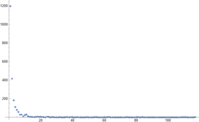
This is somewhat hard to parse, since it is so heavily weighted towards low multiplicities.
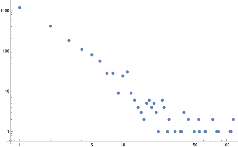
Here’s a log-log plot of the nonzero multiplicities instead:
And here is another log-log plot for $n = 10^{12}$:
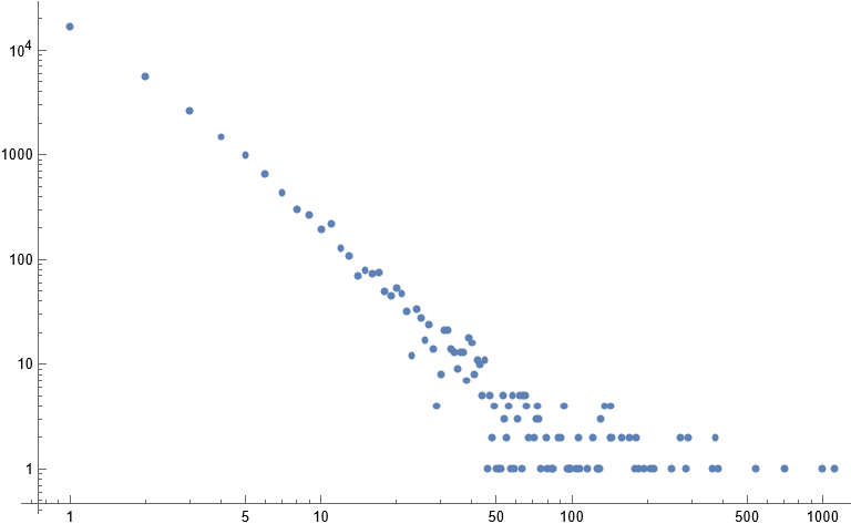
We can make the very reasonable guess that the number of slopes which are used $k$ times is bounded by something like $O(n^{1/3}\log(n)/k)$, which would give us at most $O(n^{1/3} \log(n)^2)$ trapezoids. Looking at the above plots, it seems there is some initial segment (maybe of length $O(n^{1/6})$ or something) which is nice, and then the rest becomes shallower and more chaotic. This initial segment behaves like $O(n^{1/3}\log(n)/k^2)$, which is definitely nice. If this holds for the first $n^{1/6}$ or so multiplicities, then we would get a bound of $O(n^{1/3} \log(n))$ on the number of trapezoids as desired.
Instead of thinking longer about how to prove this, let’s just move on to fixing our memory usage.
Optimizations
Memory Usage, and Slope Stack Compression
The previous data suggested that, for the hyperbola, the maximum size of the stack of slope search interval endpoints seemed to grow like $O(n^{1/3})$. Here I’ll show why it’s at least that bad.
The first steps of the algorithm will attempt to narrow the slope search interval by computing mediants between $\frac{0}{1}$ and $\frac{1}{0}$, in this case towards the steeper end. We start at around $x_0 \approx (2n)^{1/3}$.
Above is what the relevant section of the hyperbola might look like.
Given that we start at the inital point $(x_0, y_0 = 1 + \lfloor n/x_0 \rfloor)$, the stack will grow like
where finally $k$ is the largest positive integer such that $(x_0+1)(y_0-k) > n$.
Clearly if $k$ is too large this is intolerable. Indeed, back in an earlier section we dealt with an issue where $k$ was as large as $n$. The issue was that the slope near $x = 1$ was too extreme, and therefore very high slopes could fit above the blob. Naturally, the solution was to start somewhere less steep, but here that’s not really an option.
We can approximate the slope of the hyperbola at $x_0$ by
\[\frac{\mathrm d}{\mathrm dx} \frac{n}{x} = -\frac{n}{x^2} \quad \mapsto \quad -\frac{n}{(\sqrt[3]{2n})^2} = -\frac{n^{1/3}}{2^{2/3}}\]and so the initial search interval splitting is going to add $\Theta(n^{1/3})$ endpoints to our stack.
The good news is that there is a decent way of avoiding the storage of almost all of the generated endpoints, since we really only need to use the steepest one (in the case of the hyperbola) at any moment. The pattern $\left[\frac{0}{1}, \frac{1}{1}, \frac{2}{1}, \frac{3}{1}, \frac{4}{1}, \ldots, \frac{k}{1}\right]$ can be represented as a single pair
\[\left[\frac{0}{1}, \frac{1}{1}, \frac{2}{1}, \frac{3}{1}, \frac{4}{1}, \ldots, \frac{k}{1}\right] \quad \sim \quad \left[\left(\frac{k}{1}, \frac{1}{0}\right) \right]\]where the first member of the pair, $\frac{dy}{dx} = \frac{k}{1}$, is the last endpoint, and the second member $\frac{p}{q} = \frac{1}{0}$ is the right parent of $\frac{k}{1}$ in the SB tree. Or more practically, $\frac{p}{q}$ tells us the gap from $\frac{dy}{dx}$ backwards to the endpoint that precedes it. We can just happily hop backwards from $\frac{k}{1}$ all the way down to $\frac{0}{1}$ and never get lost, and everything behaves exactly how it normally would in the chull algorithm.
What if we had a more complex stack to represent?
I took the liberty of not drawing any lines from the convex hull point at the top, which I’d done in previous diagrams. The rays all get very close together and it’s hard to make out.
The slope stack, with the current strict upper bound on the slope at the right, evolves as
\[\begin{align*} &\left[\frac{0}{1}\right] & \frac{1}{0}\\ &\left[\frac{0}{1}\right] & \frac{1}{1}\\ &\left[\frac{0}{1}, \frac{1}{2}\right] & \frac{1}{1}\\ &\left[\frac{0}{1}, \frac{1}{2}\right] & \frac{2}{3}\\ &\left[\frac{0}{1}, \frac{1}{2}\right] & \frac{3}{5}\\ &\left[\frac{0}{1}, \frac{1}{2}, \frac{4}{7}\right] & \frac{3}{5}\\ &\left[\frac{0}{1}, \frac{1}{2}, \frac{4}{7}, \frac{7}{12}\right] & \frac{3}{5}\\ &\left[\frac{0}{1}, \frac{1}{2}, \frac{4}{7}, \frac{7}{12}, \frac{10}{17}\right] & \frac{3}{5}\\ \end{align*}\]Here the slope stack does not grow so large, but we can still represent the final state as
\[\left[\frac{0}{1}, \left(\frac{1}{2}, \frac{1}{1}\right), \left(\frac{10}{17}, \frac{3}{5}\right)\right]\]I’m opting to exclude the smallest member of each progression, in this case $\frac{0}{1}$ and $\frac{1}{2}$, since they are the largest member of the previous progression. This way each slope is hit once.
We’re saving basically two integers in this example, but for a much more severe case, we would be making immense savings here. The unfortunate thing is that when we’re storing a lot of endpoints implicitly, we have to do two subtractions when we want to use one. This version of the algorithm is more complicated and slightly slower. Even so, this is the way to avoid massive memory problems.
If your goal is to compute $D(n)$ for an int64 $n$, so say $n \leq 10^{18}$ or something, then you should simply let the computer store all the endpoints explicitly, if your memory allows. The requirements for these smaller $n$ are much more bearable. Even for $n = 10^{24}$ it’s still sort of ok, but if we want to compute $D(10^{30})$, which is tantalizing, it’s necessary to use some compression trick.
Here’s one way we can implement this change.
Nim Code
iterator chullConvex(x0, y0: int64,
              x1: int64,
              inside: (proc (x, y: int64): bool),
              prune: (proc (x, y, dx, dy: int64): bool)): (int64, int64, int64, int64) =
  ##Finds the convex hull of integer points
  ##with xInit <= x <= x1, and f(x) < y, where f is convex.
  ##Yields (x, y, dx, dy),
  ##where the next edge is from (x, y) to (x+dx, y-dy).
  ##(x0, y0) is the top left point of the hull, and satisfies f(x0) < y0.
  ##A point is in the shape iff inside(x, y).
  ##Also provide prune(x, y, dx, dy) which returns whether f'(x) >= -dy/dx.
  ##Note the order of the above inequality compared to chullConcave.
  ##This works for f'(x) <= 0 and f''(x) >= 0.
  #---
  var (x, y) = (x0, y0)
  var stack = @[(1'i64, 0'i64, -1'i64, -1'i64), (0'i64, 1'i64, -1'i64, -1'i64)]
  #stack of slopes (dx, dy, p, q) representing a progression of slopes
  #..., -(-2q+dy)/(-2p+dx), -(-q+dy)/(-p+dx), -dy/dx
  #if p = -1 or q = -1 then it just represents a single slope -dy/dx
  #always kept in order of shallowest slope to steepest slope
  #adjacent values form slope search intervals
  while true:
    var (dx1, dy1, p1, q1) = stack.pop()
    #(dx1, dy1) is the steepest possible slope in the convex hull
    #dx1 == 0 should never happen in the case we deal with
    #use the slope -dy1/dx1 as much as possible
    while x + dx1 <= x1 and not inside(x + dx1, y - dy1):
      yield (x, y, dx1, dy1)
      x += dx1
      y -= dy1
    #test if we are at the end already..
    #again this is not going to happen for the case we deal with
    if y == 0: break

    #get current slope search interval
    var (dx2, dy2, p2, q2) = (dx1, dy1, p1, q1)
    while stack.len != 0:
      var virtual = false #is the slope -dy1/dx1 really on the stack?
      if p2 != -1 and dx2 >= p2 and dy2 >= q2:
        virtual = true
        (dx1, dy1, p1, q1) = (dx2 - p2, dy2 - q2, p2, q2)
      else:
        (dx1, dy1, p1, q1) = stack[^1]
      #here, [dy1/dx1, dy2/dx2] forms the steepest slope search interval
      if x + dx1 <= x1 and not inside(x + dx1, y - dy1):
        break #by requirement 1, this interval contains the next slope
      #otherwise it is useless, so we discard the interval,
      #while maintaining the shallower endpoint
      if not virtual: discard stack.pop
      (dx2, dy2, p2, q2) = (dx1, dy1, p1, q1)
    if stack.len == 0: break #probably unecessary to add this here

    #the steepest slope is somewhere in [dy1/dx1,dy2/dx2]
    while true:
      var (mx, my) = (dx1 + dx2, dy1 + dy2) #interval mediant
      var usedAny = false
      while x + mx <= x1 and not inside(x + mx, y - my):
        usedAny = true
        (mx, my) = (mx + dx2, my + dy2)
      if usedAny:
        if p1 != -1 and dx1 >= p1 and dy1 >= q1:
          stack.add (dx1, dy1, p1, q1)
        #mx - dx2, my - dy2 was the last mediant that fit.
        (dx1, dy1, p1, q1) = (mx - dx2, my - dy2, dx2, dy2)
        #stack has the endpoints [..., (my-2dy2)/(mx-2dx2), (my-dy2)/(mx-dx2)] implicitly
        #active interval is [my/mx, dy2/dx2]
      else:
        if x + mx > x1 or prune(x + mx, y - my, dx1, dy1):
          #slope search prune condition
          #the intervals [dy1/dx1, (dy2+n*dy1)/(dx2+n*dx1)] never work
          #fully discard dy2/dx2 and therefore the interval [dy1/dx1, dy2/dx2]
          if p1 != -1 and dx1 >= p1 and dy1 >= q1:
            stack.add (dx1, dy1, p1, q1)
          break
        #refine the search to [dy1/dx1, my/mx]
        (dx2, dy2) = (mx, my)
        #there is no need to update p2, q2 here, as they are no longer used
    #the search is over
    #top of the stack contains the next active search interval
It’s possible to add some binary searchy type stuff in there but I’m not sure it would give you a very impressive speedup. I’ll leave that to you guys to mess around with for now, and maybe I’ll return here and add something later.
A modified version of chullConcave is also available on my GitHub.
Plugging this in for int128s was really finnicky when it came to runtime. I was able to get anywhere from about 5 seconds to as high as 8 seconds for $D(10^{20})$ depending on how many function calls and int128 initializations I could remove. Recall that the $O(n^{1/3})$ memory version needed 4.2 sec for this case.
The important bit, though, is that the low memory usage allows us to easily parallelize this version by chopping up the hyperbola into a bunch of segments. The work by Alcántara and others that I used in a previous section is useful in providing us the hueristic that we should likely split it up dyadically. My best results, however, were obtained by splitting the hyperbola at points that looked like $x = ck^3$ for a suitable constant $c$. I haven’t done any actual analysis on this so it’s probably not optimal.
I’m curious about whether GPU programming (like CUDA or something) would allow for an extremely fast implementation of this algorithm. I’m not experienced in GPU programming so I’m putting this off for now. I’ll likely investigate this some other time, but if you try it first please let me know.
Here’s a short table of data for the single-threaded version.
You’ll see the runtime is worse by a factor of about 1.3, since we’re doing more arithmetic.
| n | Max Stack Len (old) | Max Stack Len (new) | Runtime (old) | Runtime (new) | Runtime (parallelized)11 |
|---|---|---|---|---|---|
| 1020 | 2924019 | 10 | 4.2 sec | 5.4 sec | 0.6 sec |
| 1021 | 6299607 | 10 | 9.5 sec | 12 sec | 1.3 sec |
| 1022 | 13572089 | 11 | 21 sec | 28 sec | 3 sec |
| 1023 | 29240178 | 11 | 47 sec | 64 sec | 7 sec |
| 1024 | 62996054 | 11 | 107 sec | 142 sec | 15 sec |
| 1025 | 135720882 | 12 | 238 sec | 322 sec | 33 sec |
| 1026 | 292401775 | 12 | 543 sec | 697 sec | 77 sec |
| 1027 | 629960526 | 12 | 1224 sec | 1604 sec | 172 sec |
The memory optimization is wildly successful here (ignoring how much slower it is singlethreaded).
The upside of doing it this way is that the algorithm is now better suited for parallelization, as it has very little memory usage. It is in fact perfectly possible to implement this algorithm while maintaining only $O(1)$ integers instead of $O(\log n)$ of them, but I don’t see a point in doing this. I included some runtimes I got using this version of the algorithm with Int128s and splitting the hyperbola up into a bunch of chunks.
Lemma 7. The maximum stack length is $O(\log n)$.
Proof. Consider the following example state the stack can be in (given here in the convex case):
\[\left[\frac{0}{1}, \left(\frac{1}{1}, \frac{1}{0}\right), \left(\frac{3}{2}, \frac{2}{1}\right), \left(\frac{11}{7}, \frac{8}{5}\right), \left(\frac{30}{19}, \frac{19}{12}\right), \left(\frac{79}{50}, \frac{49}{31}\right), \left(\frac{207}{131}, \frac{128}{81}\right)\right]\]The avid continued fraction enjoyer would compute the sequence of convergents to $207/131$:
\[\left[\frac{0}{1}, \frac{1}{1}, \frac{2}{1}, \frac{3}{2}, \frac{8}{5}, \frac{11}{7}, \frac{19}{12}, \frac{30}{19}, \frac{49}{31}, \frac{79}{50}, \frac{207}{131}\right]\]Naturally we decide that the values in the stack correspond to some of the convergents to a rational number.
The number of convergents for a rational number $dy/dx$ with $dx, dy \leq n$ is $O(\log n)$.
I don’t really want to go into it in much more detail, if you’re curious I’ll again recommend the blog by adamant and the page on the Stern Brocot tree. This is good enough for now. $\proofqed$
The highest value $D(10^n)$ I’ve seen computed was $D(10^{36})$.
This approach would take about 65 hours to get this value.
Next Time
I’m cutting the article off here for now, but I have some other topics I want to get to later.
The most important of those is computing big partial sums of $\sigma_1$, which is done in the same way except we need some more difficult sums over the trapezoids. Min25 mentions how to do it basically, but I’ll outline it in a followup blog post once I actually implement it myself.
I also want to review how these methods can be used to count solutions to some quadratic diophantine equations, to count powerful numbers up to some huge limit (maybe, I’m still wrestling bigint operations), and computing $\pi(n) \bmod 2$. I’ll include those in the followup later if they work out.
Appendix
What if we did want to compute the sum $R(n)$ with multiplicative functions?
I only just started writing this article and I’m already distracted, oh no.
Anyways, for $k > 0$, $r_2(k)$ actually is $4$ times a multiplicative function in $k$.
I’ll go ahead and write $r_2(k) = 4g(k)$ for $k > 0$.
It happens that $g(k)$ is the number of divisors of $k$ which are $1$ mod $4$ minus the number of divisors which are $3$ mod $4$. We can write this as $g(k) = \sum_{d \mid k} \chi(d)$, where $\chi$ is the nontrivial Dirichlet character modulo 4. In other words, $\chi$ is the periodic function whose values begin as $1, 0, -1, 0$, and so on repeating.
Now we can use the hyperbola method on $g = u \ast \chi$ compute it in $O(\sqrt{n})$ terms as
\[R(n) = 1 + 4\left[\sum_{k \leq \sqrt{n}} X(n/k) + \sum_{k \leq \sqrt{n}} \chi(k) \left\lfloor \frac{n}{k} \right\rfloor - X(\sqrt{n})\lfloor \sqrt{n}\rfloor\right]\]where $X(n) = \sum_{k \leq n} \chi(n)$ is also periodic, whose values begin as $1, 1, 0, 0$ and so on.
We can implement it as
proc R(n: int64): int64 =
  let sqrtn = isqrt(n)
  for k in 1..sqrtn:
    result += [0, 1, 1, 0][(n div k) mod 4]
    result += [0, 1, 0, -1][k mod 4] * (n div k)
  result -= [0, 1, 1, 0][sqrtn mod 4] * sqrtn
  return 1 + 4*result
You can think about this longer and eventually get $\frac{\pi}{4} = 1 - \frac{1}{3} + \frac{1}{5} - \frac{1}{7} + \ldots$ if you want.
Code
The code for this blog post is available here on GitHub.
Thanks to Ann, hacatu, and shash4321 for proofreading this and giving good feedback.
-
Obviously the reason is that we are using $(x, y)$ as coordinates on a grid, and I would rather avoid the confusion. So from here on, we will be using $n$ as our summation limit, and $k$ as the free variable in the summation. The letters $x, y$ will always be used to refer to some sort of coordinates. ↩
-
I made all the diagrams on this page by hand in Aseprite. The hyperbola is a Bézier curve with points at $(1, 16), (2, 3), (3, 2), (16, 1)$. ↩
-
Unless you’re extremely patient. For $n = 10^{24}$ I estimated something like over two hours runtime for this more basic algorithm. It is pretty parallelizable though, if you’re exceptionally lazy, since it has no memory requirement. ↩
-
Or into trapeziums if you’re British. ↩
-
Actually you probably don’t need $x$, but later you might be counting points of a specific form inside the trapezoid for which you may want information about the $x$ value. ↩
-
Which is how I was attempting to do it while writing this, until I realized I hated it when I had to debug a ton of stuff forever and never got it to work nicely in a way that made sense and was easy to communicate ↩
-
We can consider $(0, -1)$ to be the steepest vector, and $(1, 0)$ to be the shallowest. So really we’re finding $(dx, -dy)$ such that $dy/dx$ is as low as possible, and such that $(x+dx, y-dy)$ fits in the blob. ↩
-
It is ↩
-
This was unnecessarily confusing honestly. A convex function is one where the set of points ABOVE it form a convex set. This is why we have to flip it upside down in that case. A concave function is one where the points underneath it form a convex set, which is the case for the circle function. ↩
-
The convex lattice polygon on the right contains exactly one interior point. It is a representative of one of the 16 equivalence classes of convex lattice polygons which contain only one interior point, up to lattice equivalence. Very curious.. see this other Rabinowitz paper to see more about that. ↩
-
I also avoided some int128 multiplications here for a bit better performance, but it’s by no means completely optimized. This is just to get an idea of how fast we can make this. I computed these using an AMD Ryzen 3700x. ↩